A Simple Optimization Problem

Formulate and solve a one-dimensional constrained minimization problem.

Author

Samer El Kababji

Published

October 24, 2026

Setup

This notebook requires Python 3.11, NumPy, and Matplotlib. Run this command in a notebook cell once if they are not already installed:

%pip install matplotlib==3.10.8 numpy==2.2.6

Restart the kernel after installation, then run the notebook from top to bottom.

%matplotlib inline
import matplotlib.pyplot as plt
import numpy as np

Learning objectives

By the end of this notebook, you will be able to:

distinguish an objective function from a constraint;
identify the feasible set of an optimization problem;
solve a simple constrained problem analytically; and
verify the solution numerically and graphically.

1. State the problem

Consider the constrained optimization problem

\[ \begin{aligned} \text{minimize}_{x\in\mathbb{R}}\quad & f(x)=(x-3)^2 \\ \text{subject to}\quad & x\leq 1. \end{aligned} \]

The objective \(f(x)\) measures squared distance from \(3\). Without the constraint its minimum is at \(x=3\), but \(3\) is infeasible. The feasible set is \((-\infty,1]\).

2. Solve it analytically

The derivative of the objective is \(f'(x)=2(x-3)\). For every feasible \(x\leq1\), this derivative is negative, so \(f\) decreases as \(x\) moves right. The best feasible point is therefore the boundary:

\[x^\star=1,\qquad p^\star=f(1)=4.\]

Here \(x^\star\) is the optimizer and \(p^\star\) is the optimal value.

x = np.linspace(-2, 5, 500)
f = (x - 3) ** 2

fig, ax = plt.subplots(figsize=(8, 5))
ax.plot(x, f, color="#047857", linewidth=2, label=r"$f(x)=(x-3)^2$")
ax.axvspan(x.min(), 1, color="#6ee7b7", alpha=0.25, label=r"feasible: $x\leq1$")
ax.axvline(1, color="#065f46", linestyle="--", linewidth=1.5)
ax.scatter([1], [4], color="#b45309", s=90, zorder=4, label=r"$(x^\star,p^\star)=(1,4)$")
ax.scatter([3], [0], facecolors="none", edgecolors="#374151", s=90, label="unconstrained minimum")
ax.set(xlabel="x", ylabel="f(x)", title="A constrained quadratic minimization problem", ylim=(-1, 26))
ax.legend()
ax.grid(alpha=0.2)
plt.show()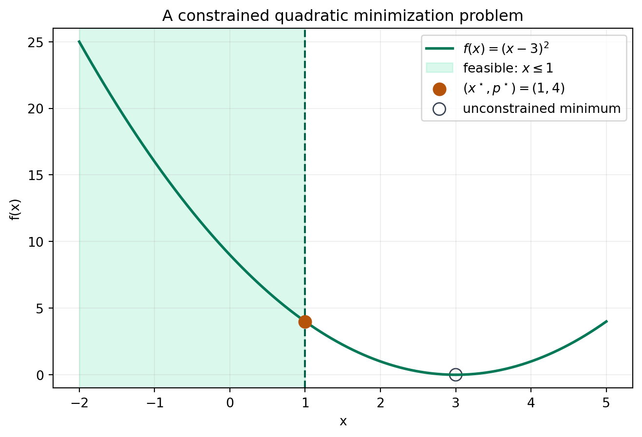

Figure 1: The constrained minimum occurs where the feasible region ends.

3. Verify it numerically

A dense grid is not a general optimization algorithm, but it makes a useful check in one dimension.

x_feasible = np.linspace(-10, 1, 20_001)
objective_values = (x_feasible - 3) ** 2
best_index = np.argmin(objective_values)

x_star = x_feasible[best_index]
p_star = objective_values[best_index]
print(f"optimizer x*    = {x_star:.3f}")
print(f"optimal value p* = {p_star:.3f}")

optimizer x*    = 1.000
optimal value p* = 4.000

4. What to remember

An optimization problem has an objective, decision variables, and possibly constraints. A constraint can move the optimum away from the unconstrained stationary point and onto the boundary of the feasible set.

In the next notebook, we will recover the same value \(p^\star=4\) from a dual maximization problem.

Exercises

Replace the constraint by \(x\leq2\). Predict the optimizer before rerunning the code.
Replace the constraint by \(x\leq4\). Is the constraint active at the solution?
Replace the objective by \((x-a)^2\) and describe the optimizer as a function of \(a\).