Support Vector Machines

The geometry and mathematics of maximum-margin classification, built step by step from first principles.

Author

Samer El Kababji

Published

October 24, 2026

Setup

This notebook requires Python 3.11 and the packages below. Run this command in a notebook cell once if they are not already installed:

%pip install matplotlib==3.10.8 numpy==2.2.6 scikit-learn==1.7.2

Restart the kernel after installation, then run the notebook from top to bottom.

%matplotlib inline
import matplotlib.pyplot as plt
import numpy as np
from sklearn.datasets import make_blobs, make_moons
from sklearn.preprocessing import StandardScaler
from sklearn.svm import SVC

RANDOM_SEED = 7
np.random.seed(RANDOM_SEED)

Learning goals

By the end of this lesson, you should be able to:

state the maximum-margin criterion and express it as a constrained optimisation;
read and interpret the primal and dual forms of the SVM;
explain what a support vector is and why only a few observations determine the boundary; and
recognise the role of the regularisation parameter \(C\) in soft-margin classification.

1. The separating hyperplane

Given a binary dataset

\[ \mathcal{D}=\{(\mathbf{x}_i,y_i)\}_{i=1}^{N}, \qquad \mathbf{x}_i\in\mathbb{R}^d,\quad y_i\in\{-1,+1\}, \]

a linear classifier assigns labels via the signed decision function

\[ f(\mathbf{x}) = \operatorname{sign}\!\bigl(\mathbf{w}^\top\mathbf{x}+b\bigr), \]

where \(\mathbf{w}\in\mathbb{R}^d\) is the weight vector and \(b\in\mathbb{R}\) is the bias.
The set of points satisfying \(\mathbf{w}^\top\mathbf{x}+b=0\) is the decision hyperplane.

For a refresher on line equations and basic vector analysis, see 1.1 Margin Geometry.

X, y = make_blobs(n_samples=60, centers=2, cluster_std=0.8, random_state=RANDOM_SEED)
y = 2 * y - 1  # map {0, 1} to {-1, +1}

X = StandardScaler().fit_transform(X)

fig, ax = plt.subplots(figsize=(6, 5))
for lbl, color in [(-1, '#3157a4'), (1, '#e07a3f')]:
    ax.scatter(*X[y == lbl].T, c=color, label=f'y = {lbl}')
ax.set(xlabel='$x_1$', ylabel='$x_2$', title='Two-class dataset')
ax.legend()
plt.show()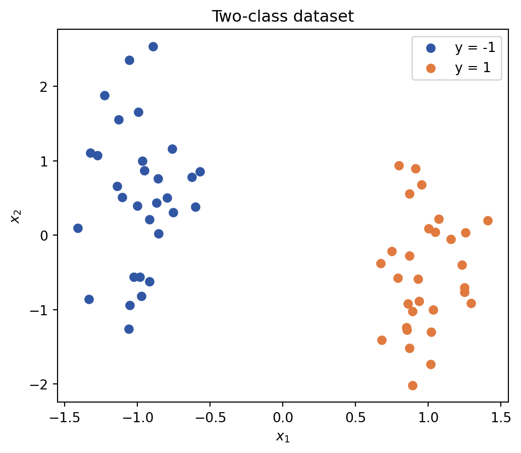

Figure 1: A two-class dataset whose classes are linearly separable.

2. Maximizing the margin

Among all separating hyperplanes, the SVM selects the one that maximises the geometric margin—the perpendicular distance from the hyperplane to the nearest observation on each side.

Rescaling \(\mathbf{w}\) and \(b\) so that the closest observations satisfy

\[ y_i\bigl(\mathbf{w}^\top\mathbf{x}_i+b\bigr)\geq 1, \]

Prove it!

the two margin hyperplanes are \(\mathbf{w}^\top\mathbf{x}+b=\pm 1\), and the geometric margin equals \(\dfrac{2}{\lVert\mathbf{w}\rVert}\).

Maximising the margin is therefore equivalent to the primal problem (hard margin):

\[ \min_{\mathbf{w},\,b}\;\frac{1}{2}\lVert\mathbf{w}\rVert^2 \qquad\text{subject to}\quad y_i\bigl(\mathbf{w}^\top\mathbf{x}_i+b\bigr)\geq 1,\quad i=1,\ldots,N. \]

model = SVC(kernel='linear', C=1e6)   # large C approximates the hard-margin SVM
model.fit(X, y)

w = model.coef_[0]
b = model.intercept_[0]
margin = 2 / np.linalg.norm(w)

x1 = np.linspace(X[:, 0].min() - 0.5, X[:, 0].max() + 0.5, 300)
x2_mid = (-b      - w[0] * x1) / w[1]
x2_pos = ( 1 - b  - w[0] * x1) / w[1]
x2_neg = (-1 - b  - w[0] * x1) / w[1]

fig, ax = plt.subplots(figsize=(6, 5))
for lbl, color in [(-1, '#3157a4'), (1, '#e07a3f')]:
    ax.scatter(*X[y == lbl].T, c=color, label=f'y = {lbl}', zorder=3)
ax.scatter(
    *X[model.support_].T,
    s=180, facecolors='none', edgecolors='k', linewidths=1.5,
    label='support vectors', zorder=4,
)
ax.plot(x1, x2_mid, 'k-',  label='decision boundary')
ax.plot(x1, x2_pos, 'k--', alpha=0.5, label='margin hyperplanes')
ax.plot(x1, x2_neg, 'k--', alpha=0.5)
ax.fill_between(x1, x2_neg, x2_pos, alpha=0.10, color='gray', label='margin')
ax.set(xlabel='$x_1$', ylabel='$x_2$',
       title=f'Maximum-margin hyperplane  (margin = {margin:.3f})')
ax.legend(fontsize=8)
plt.show()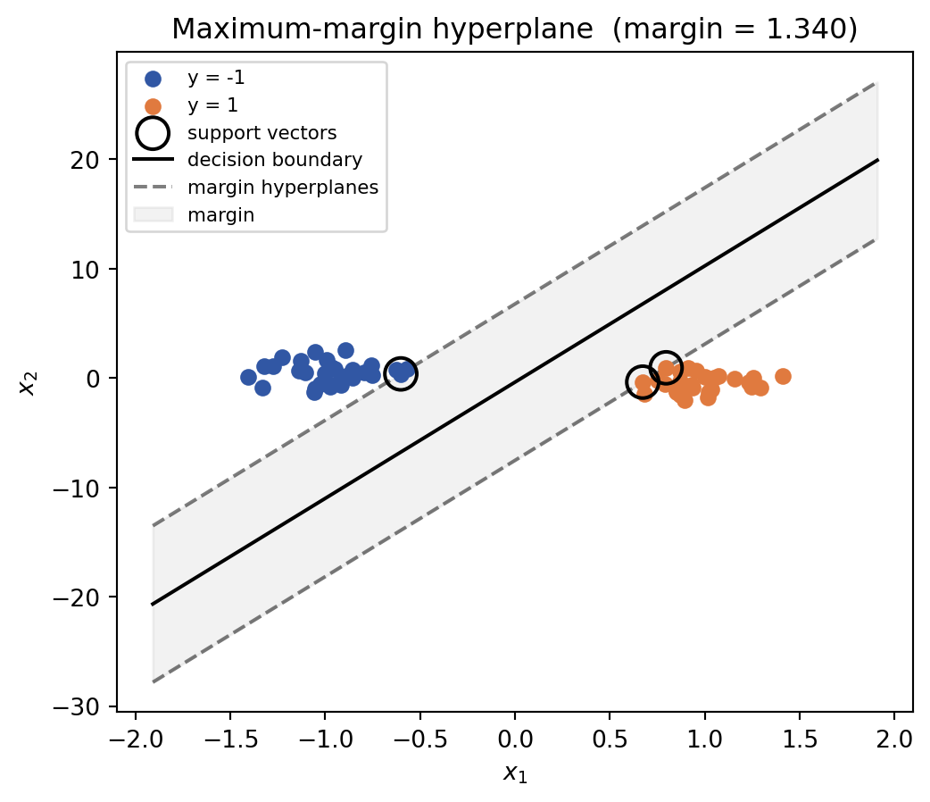

Figure 2: Maximum-margin hyperplane with margin band and support vectors circled.

3. The dual problem

Introducing a Lagrange multiplier \(\alpha_i\geq 0\) for each constraint, the Lagrangian is

\[ L(\mathbf{w},b,\boldsymbol{\alpha}) =\frac{1}{2}\lVert\mathbf{w}\rVert^2 -\sum_{i=1}^{N}\alpha_i\bigl[y_i(\mathbf{w}^\top\mathbf{x}_i+b)-1\bigr]. \]

Setting \(\partial L/\partial\mathbf{w}=\mathbf{0}\) and \(\partial L/\partial b=0\) yields

\[ \mathbf{w}=\sum_{i=1}^{N}\alpha_i y_i\mathbf{x}_i, \qquad \sum_{i=1}^{N}\alpha_i y_i=0. \]

Substituting back gives the dual problem:

\[ \max_{\boldsymbol{\alpha}}\;\sum_{i=1}^{N}\alpha_i -\frac{1}{2}\sum_{i=1}^{N}\sum_{j=1}^{N} \alpha_i\alpha_j y_i y_j\,\mathbf{x}_i^\top\mathbf{x}_j \qquad\text{subject to}\quad \alpha_i\geq 0,\quad\sum_{i=1}^{N}\alpha_i y_i=0. \]

By the KKT conditions, \(\alpha_i>0\) only for observations on the margin hyperplanes—the support vectors. All other \(\alpha_i=0\).

print(f'Total observations : {len(y)}')
print(f'Support vectors    : {len(model.support_)}')

# model.dual_coef_ stores alpha_i * y_i; reconstruct w = sum_i alpha_i y_i x_i
w_dual = (model.dual_coef_ @ model.support_vectors_).ravel()

print(f'\nw from dual : {np.round(w_dual, 5)}')
print(f'w from coef_: {np.round(model.coef_[0], 5)}')

Total observations : 60
Support vectors    : 3

w from dual : [ 1.4861  -0.13975]
w from coef_: [ 1.4861  -0.13975]

4. Soft-margin SVM

Real datasets are rarely linearly separable. Introducing slack variables \(\xi_i\geq 0\) allows observations to be inside or on the wrong side of the margin while penalising those violations:

\[ \min_{\mathbf{w},\,b,\,\boldsymbol{\xi}}\; \frac{1}{2}\lVert\mathbf{w}\rVert^2+C\sum_{i=1}^{N}\xi_i \qquad\text{subject to}\quad y_i\bigl(\mathbf{w}^\top\mathbf{x}_i+b\bigr)\geq 1-\xi_i,\quad \xi_i\geq 0. \]

The parameter \(C>0\) governs the trade-off between margin width and training error:

\(C\)	margin	misclassifications
small	wide	many tolerated
large	narrow	few tolerated

X_s, y_s = make_moons(n_samples=80, noise=0.25, random_state=RANDOM_SEED)
y_s = 2 * y_s - 1

xx, yy = np.meshgrid(
    np.linspace(-1.5, 2.5, 300),
    np.linspace(-1.5, 2.0, 300),
)

fig, axes = plt.subplots(1, 3, figsize=(14, 4), sharey=True)
for ax, C in zip(axes, [0.1, 1.0, 100.0]):
    clf = SVC(kernel='linear', C=C)
    clf.fit(X_s, y_s)
    Z = clf.predict(np.c_[xx.ravel(), yy.ravel()]).reshape(xx.shape)

    ax.contourf(xx, yy, Z, alpha=0.15, cmap='coolwarm')
    ax.contour(xx, yy, Z, colors='k', linewidths=0.8)
    for lbl, color in [(-1, '#3157a4'), (1, '#e07a3f')]:
        ax.scatter(*X_s[y_s == lbl].T, c=color, s=25)
    ax.scatter(
        *X_s[clf.support_].T,
        s=100, facecolors='none', edgecolors='k', linewidths=1.2,
    )
    ax.set_title(f'C = {C}  |  {len(clf.support_)} SVs', fontsize=10)
    ax.set_xlabel('$x_1$')
axes[0].set_ylabel('$x_2$')
fig.suptitle('Effect of C on the soft-margin decision boundary', fontsize=11)
plt.tight_layout()
plt.show()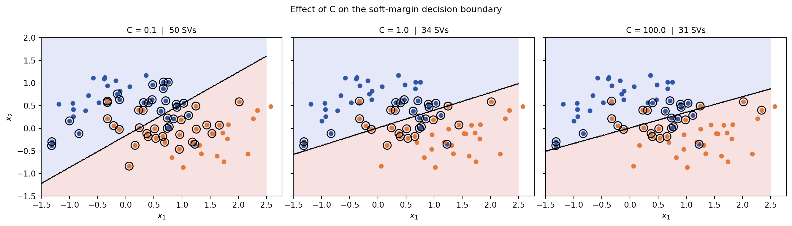

Figure 3: Decision boundaries and support-vector counts for three values of C.

Try it yourself

Change RANDOM_SEED and rerun every cell. Do the same support vectors appear?
Increase cluster_std in make_blobs. At what value does the hard-margin SVM start to struggle?
In the soft-margin experiment, raise noise in make_moons to 0.40. How does \(C\) change the support-vector count?
Set C = 1.0 and switch to kernel='poly' with degree=2. How does the boundary shape change?