import matplotlib.pyplot as plt
import numpy as np
from sklearn.datasets import make_moons
from sklearn.metrics import accuracy_score
from sklearn.model_selection import train_test_split
from sklearn.preprocessing import MinMaxScaler
from sklearn.svm import SVC

RANDOM_SEED = 7
np.random.seed(RANDOM_SEED)
SVM: Classical and quantum kernel classifiers
A mathematical and computational comparison using the same data and support-vector learning rule.
Setup
This notebook requires Python 3.11 and the packages below. Run this command in a notebook cell once if they are not already installed:
%pip install matplotlib==3.10.8 numpy==2.2.6 pandas==2.3.3 qiskit==2.2.3 qiskit-machine-learning==0.9.0 scikit-learn==1.7.2Restart the kernel after installation, then run the notebook from top to bottom. No quantum-hardware account is required.
Learning goals
By the end of this lesson, you should be able to:
- explain how a kernel measures similarity;
- distinguish a classical feature map from a quantum feature map;
- train both classifiers on the same data; and
- interpret the comparison without claiming a quantum advantage.
Note
This notebook assumes familiarity with SVMs and kernel functions. If you are new to these topics, read the Support Vector Machines and Kernels in SVMs notebooks first.
Important
This notebook runs the quantum circuit on a classical statevector simulator. It is a teaching example, not a performance benchmark or evidence of quantum advantage.
1. The classification problem
A binary classification dataset contains feature vectors and labels
\[ \mathcal{D}=\{(\mathbf{x}_i,y_i)\}_{i=1}^{N}, \qquad \mathbf{x}_i\in\mathbb{R}^d,\quad y_i\in\{0,1\}. \]
A classifier learns a function \(f:\mathbb{R}^d\rightarrow\{0,1\}\) from a training subset. We evaluate it on data that was not used for fitting.
X, y = make_moons(n_samples=50, noise=0.12, random_state=RANDOM_SEED)
X = MinMaxScaler(feature_range=(0, np.pi)).fit_transform(X)
X_train, X_test, y_train, y_test = train_test_split(
    X, y, test_size=0.30, stratify=y, random_state=RANDOM_SEED
)

fig, ax = plt.subplots(figsize=(7, 5))
for label, color in [(0, "#3157a4"), (1, "#e07a3f")]:
    ax.scatter(*X_train[y_train == label].T, c=color, marker="o", label=f"class {label}: train")
    ax.scatter(*X_test[y_test == label].T, c=color, marker="x", s=70, label=f"class {label}: test")
ax.set(xlabel="$x_1$", ylabel="$x_2$", title="Two-class dataset")
ax.legend(ncols=2, fontsize=8)
plt.show()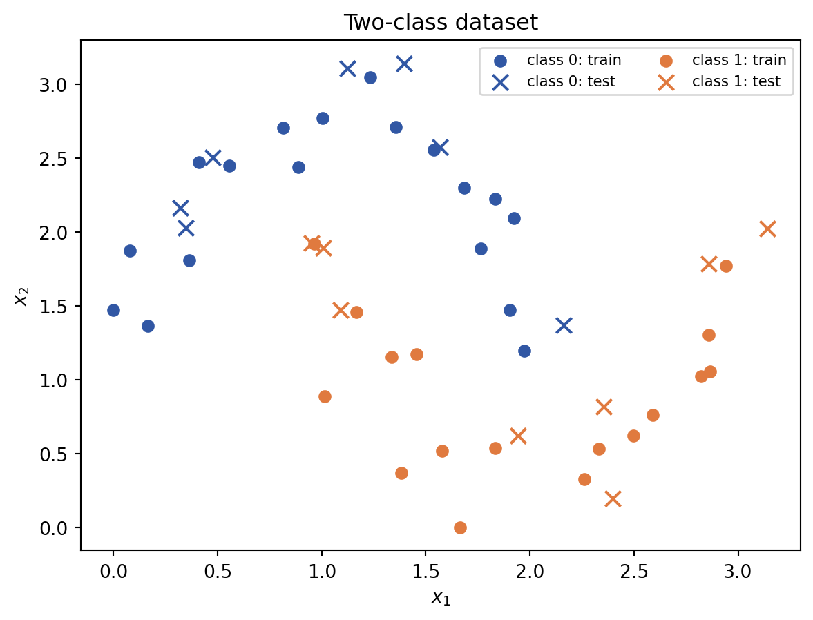
2. Classical kernel classifier
A kernel computes similarity without requiring us to explicitly construct every coordinate of a feature map \(\phi\):
\[ k(\mathbf{x},\mathbf{z}) =\langle\phi(\mathbf{x}),\phi(\mathbf{z})\rangle. \]
We use the radial-basis-function kernel
\[ k_{\mathrm{RBF}}(\mathbf{x},\mathbf{z}) =\exp\!\left(-\gamma\lVert\mathbf{x}-\mathbf{z}\rVert^2\right). \]
Nearby observations have a kernel value close to \(1\); distant observations have a value closer to \(0\).
classical_model = SVC(kernel="rbf", gamma="scale")
classical_model.fit(X_train, y_train)
classical_predictions = classical_model.predict(X_test)
classical_accuracy = accuracy_score(y_test, classical_predictions)

print(f"Classical test accuracy: {classical_accuracy:.3f}")
Classical test accuracy: 0.8003. Quantum feature map and kernel
A parameterized quantum circuit \(U_\phi(\mathbf{x})\) encodes a classical vector as a quantum state:
\[ |\phi(\mathbf{x})\rangle =U_\phi(\mathbf{x})|0\rangle^{\otimes n}. \]
The quantum kernel is the squared overlap between two encoded states:
\[ k_Q(\mathbf{x},\mathbf{z}) =\left|\langle\phi(\mathbf{x})|\phi(\mathbf{z})\rangle\right|^2. \]
The support-vector optimization remains classical. The quantum part supplies the kernel matrix.
from qiskit.circuit.library import zz_feature_map

feature_map = zz_feature_map(feature_dimension=2, reps=2, entanglement="linear")
print(feature_map.draw(output="text", fold=90))
┌───┐┌───────────┐ ┌───┐┌───────────┐ »
0: ┤ H ├┤ P(2*x[0]) ├──■────────────────────────────────────■──┤ H ├┤ P(2*x[0]) ├──■──»
├───┤├───────────┤┌─┴─┐┌──────────────────────────────┐┌─┴─┐├───┤├───────────┤┌─┴─┐»
1: ┤ H ├┤ P(2*x[1]) ├┤ X ├┤ P((-π + x[0])*(-π + x[1])*2) ├┤ X ├┤ H ├┤ P(2*x[1]) ├┤ X ├»
└───┘└───────────┘└───┘└──────────────────────────────┘└───┘└───┘└───────────┘└───┘»
«
«0: ──────────────────────────────────■──
« ┌──────────────────────────────┐┌─┴─┐
«1: ┤ P((-π + x[0])*(-π + x[1])*2) ├┤ X ├
« └──────────────────────────────┘└───┘from qiskit_machine_learning.algorithms import QSVC
from qiskit_machine_learning.kernels import FidelityStatevectorKernel
# Exact classical simulation of quantum states: no hardware account required.
quantum_kernel = FidelityStatevectorKernel(feature_map=feature_map)
quantum_model = QSVC(quantum_kernel=quantum_kernel)
quantum_model.fit(X_train, y_train)
quantum_predictions = quantum_model.predict(X_test)
quantum_accuracy = accuracy_score(y_test, quantum_predictions)
print(f"Quantum-kernel test accuracy: {quantum_accuracy:.3f}")Quantum-kernel test accuracy: 0.8674. Inspect the quantum kernel matrix
For training observations \(\mathbf{x}_1,\ldots,\mathbf{x}_m\), the matrix
\[ K_{ij}=k_Q(\mathbf{x}_i,\mathbf{x}_j) \]
contains every pairwise similarity supplied to the support-vector algorithm. The diagonal is \(1\) because each state has perfect overlap with itself.
K_train = quantum_kernel.evaluate(X_train)
fig, ax = plt.subplots(figsize=(6, 5))
image = ax.imshow(K_train, vmin=0, vmax=1, cmap="viridis")
ax.set(xlabel="training observation $j$", ylabel="training observation $i$")
fig.colorbar(image, ax=ax, label="$K_{ij}$")
plt.show()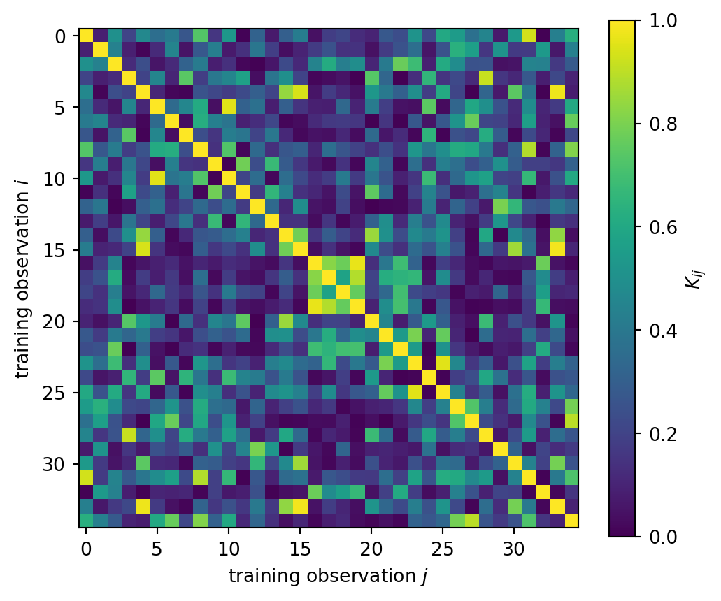
5. Compare the results
Accuracy is
\[ \operatorname{accuracy} =\frac{\text{number of correct predictions}} {\text{number of test observations}}. \]
Because this test set is deliberately small, one changed prediction can noticeably change the score. Treat the result as an illustration, not a general ranking.
import pandas as pd

comparison = pd.DataFrame(
    {
        "classifier": ["Classical RBF SVC", "Quantum-kernel QSVC"],
        "test accuracy": [classical_accuracy, quantum_accuracy],
        "kernel source": ["Classical formula", "Simulated two-qubit circuit"],
    }
)
comparison| classifier | test accuracy | kernel source | |
|---|---|---|---|
| 0 | Classical RBF SVC | 0.800000 | Classical formula |
| 1 | Quantum-kernel QSVC | 0.866667 | Simulated two-qubit circuit |
What can we conclude?
- Both models use the same observations, split, labels, and support-vector learning principle.
- They differ in how similarity is computed.
- The quantum model is simulated by a classical computer here, so it cannot provide a runtime advantage.
- A result on one tiny dataset does not establish that either kernel is generally superior.
Try it yourself
- Change
RANDOM_SEEDand rerun every cell. - Increase
noiseinmake_moons. - Change the feature-map repetitions from
reps=2toreps=1orreps=3. - Record how accuracy and the quantum kernel matrix change.
These experiments separate stable mathematical definitions from results that depend on data and modeling choices.