Kernels in Support Vector Machines

How kernel functions implicitly map observations into higher-dimensional spaces where linear separation becomes possible.

Author

Samer El Kababji

Published

October 24, 2026

Setup

This notebook requires Python 3.11 and the packages below. Run this command in a notebook cell once if they are not already installed:

%pip install matplotlib==3.10.8 numpy==2.2.6 scikit-learn==1.7.2

Restart the kernel after installation, then run the notebook from top to bottom.

%matplotlib inline
import matplotlib.pyplot as plt
import numpy as np
from sklearn.datasets import make_circles
from sklearn.metrics.pairwise import rbf_kernel, polynomial_kernel
from sklearn.svm import SVC

RANDOM_SEED = 7
np.random.seed(RANDOM_SEED)

Learning goals

By the end of this lesson, you should be able to:

explain why some datasets cannot be separated by a hyperplane in the original feature space;
define a feature map \(\phi\) and describe what it does geometrically;
state the kernel trick and explain how it avoids computing \(\phi(\mathbf{x})\) explicitly;
identify the RBF and polynomial kernels and describe their parameters; and
write the kernel SVM decision function in terms of support vectors and the kernel.

Note

This lesson assumes familiarity with the SVM margin and dual formulation covered in the Support Vector Machines notebook.

1. When a linear classifier fails

A hyperplane in \(\mathbb{R}^d\) can correctly separate two classes only when they are linearly separable. Consider a binary dataset

\[ \mathcal{D}=\{(\mathbf{x}_i,y_i)\}_{i=1}^{N}, \qquad \mathbf{x}_i\in\mathbb{R}^d,\quad y_i\in\{-1,+1\}. \]

For a concentric-ring layout, the signed decision function \(f(\mathbf{x})=\operatorname{sign}(\mathbf{w}^\top\mathbf{x}+b)\) will misclassify some observations for every choice of \(\mathbf{w}\) and \(b\).

X, y = make_circles(n_samples=100, noise=0.10, factor=0.4, random_state=RANDOM_SEED)
y = 2 * y - 1  # map {0, 1} to {-1, +1}

xx, yy = np.meshgrid(np.linspace(-1.5, 1.5, 300), np.linspace(-1.5, 1.5, 300))
clf_lin = SVC(kernel='linear', C=1.0)
clf_lin.fit(X, y)
Z_lin = clf_lin.predict(np.c_[xx.ravel(), yy.ravel()]).reshape(xx.shape)

fig, axes = plt.subplots(1, 2, figsize=(12, 5))

ax = axes[0]
for lbl, color in [(-1, '#3157a4'), (1, '#e07a3f')]:
    ax.scatter(*X[y == lbl].T, c=color, label=f'y = {lbl}')
ax.set(xlabel='$x_1$', ylabel='$x_2$', title='Original feature space', aspect='equal')
ax.legend()

ax2 = axes[1]
ax2.contourf(xx, yy, Z_lin, alpha=0.15, cmap='coolwarm')
ax2.contour(xx, yy, Z_lin, colors='k', linewidths=0.8)
for lbl, color in [(-1, '#3157a4'), (1, '#e07a3f')]:
    ax2.scatter(*X[y == lbl].T, c=color, s=25)
acc_lin = (clf_lin.predict(X) == y).mean()
ax2.set(xlabel='$x_1$', ylabel='$x_2$',
        title=f'Linear SVM (train accuracy = {acc_lin:.0%})', aspect='equal')

plt.tight_layout()
plt.show()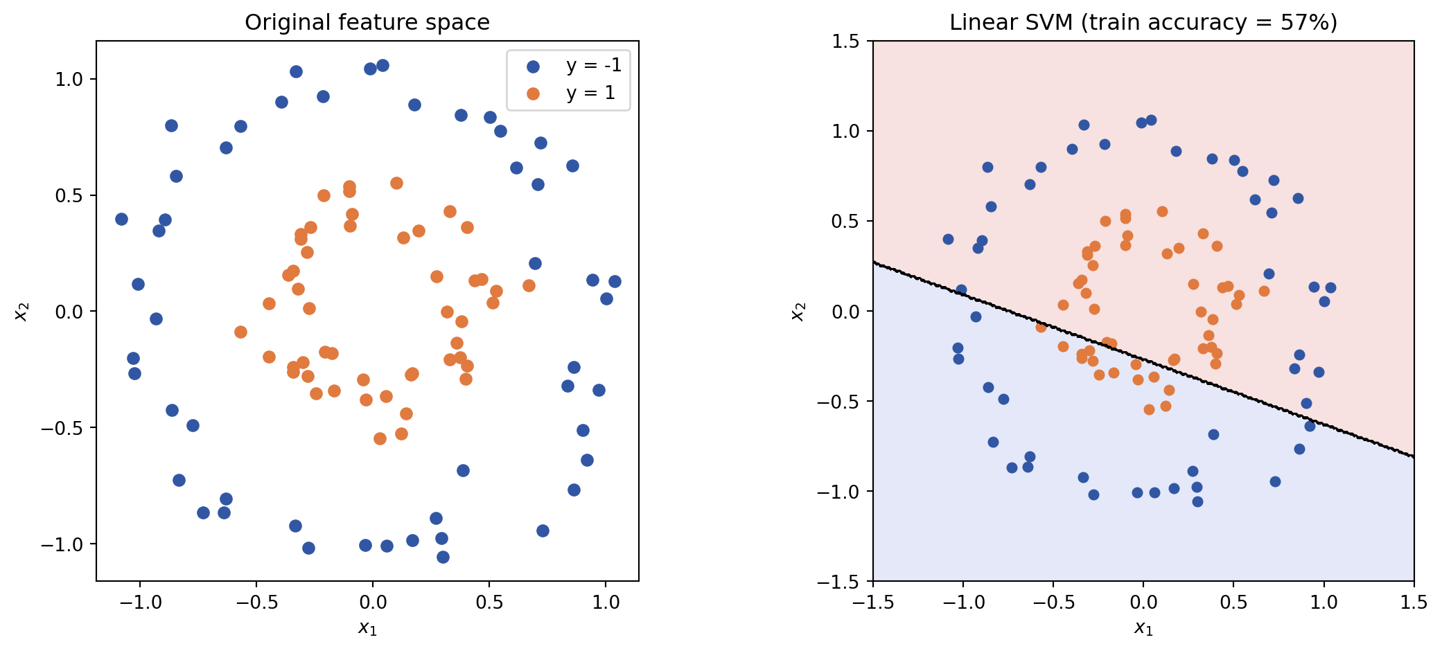

Figure 1: Concentric rings: no hyperplane separates the two classes.

2. Feature maps

A feature map \(\phi\) lifts each observation from \(\mathbb{R}^d\) into a (possibly higher-dimensional) Hilbert space \(\mathcal{H}\):

\[ \phi:\mathbb{R}^d\to\mathcal{H}. \]

Choosing \(\phi\) so that the lifted observations are linearly separable allows the standard linear SVM to operate in \(\mathcal{H}\).

Example. For \(d=2\), define the degree-2 polynomial feature map

\[ \phi(x_1,x_2) =\bigl(x_1^2,\;\sqrt{2}\,x_1 x_2,\;x_2^2\bigr)\in\mathbb{R}^3. \]

After this lift, the two concentric rings become linearly separable by a plane in \(\mathbb{R}^3\).

def phi_poly2(Xin):
    u, v = Xin[:, 0], Xin[:, 1]
    return np.column_stack([u**2, np.sqrt(2) * u * v, v**2])

X_lifted = phi_poly2(X)

fig = plt.figure(figsize=(7, 5))
ax3d = fig.add_subplot(111, projection='3d')
for lbl, color in [(-1, '#3157a4'), (1, '#e07a3f')]:
    ax3d.scatter(*X_lifted[y == lbl].T, c=color, label=f'y = {lbl}', alpha=0.7)
ax3d.set_xlabel('x1**2')
ax3d.set_ylabel('sqrt2 * x1 * x2')
ax3d.set_zlabel('x2**2')
ax3d.set_title('Degree-2 polynomial feature space')
ax3d.legend()
plt.show()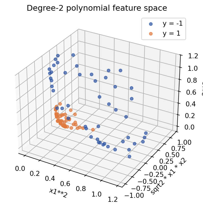

Figure 2: After the polynomial feature map, the two rings are linearly separable.

3. The kernel trick

Constructing \(\phi(\mathbf{x})\) explicitly can be expensive or impossible when \(\mathcal{H}\) is infinite-dimensional. The kernel trick observes that the SVM dual depends on \(\phi\) only through inner products \(\langle\phi(\mathbf{x}),\phi(\mathbf{z})\rangle_{\mathcal{H}}\).

A kernel function computes this inner product directly, without ever forming \(\phi\):

\[ k(\mathbf{x},\mathbf{z}) =\langle\phi(\mathbf{x}),\phi(\mathbf{z})\rangle_{\mathcal{H}}. \]

Two widely used kernels are:

Kernel	Formula	Parameter
Polynomial	\(k_\mathrm{poly}(\mathbf{x},\mathbf{z})=(1+\mathbf{x}^\top\mathbf{z})^p\)	degree \(p\)
RBF (Gaussian)	\(k_\mathrm{RBF}(\mathbf{x},\mathbf{z})=\exp\!\left(-\gamma\lVert\mathbf{x}-\mathbf{z}\rVert^2\right)\)	bandwidth \(\gamma\)

The RBF kernel corresponds to an infinite-dimensional feature space; \(k_\mathrm{RBF}\) is a simple closed-form expression that sidesteps the need to construct that space.

The matrix \(K\in\mathbb{R}^{N\times N}\) with entries \(K_{ij}=k(\mathbf{x}_i,\mathbf{x}_j)\) is the kernel matrix (also called the Gram matrix). It encodes all pairwise similarities needed by the SVM optimiser.

idx = np.argsort(y)
X_sorted = X[idx]

K_rbf  = rbf_kernel(X_sorted, gamma=1.0)
K_poly = polynomial_kernel(X_sorted, degree=2, coef0=1)
K_poly = K_poly / K_poly.max()  # normalise for display

fig, axes = plt.subplots(1, 2, figsize=(11, 4))
for ax, K, title in zip(
    axes,
    [K_rbf, K_poly],
    ['RBF kernel  (gamma = 1)', 'Polynomial kernel, degree 2 (normalised)'],
):
    img = ax.imshow(K, cmap='viridis', vmin=0, vmax=1)
    ax.set(xlabel='observation j', ylabel='observation i', title=title)
    fig.colorbar(img, ax=ax)
plt.tight_layout()
plt.show()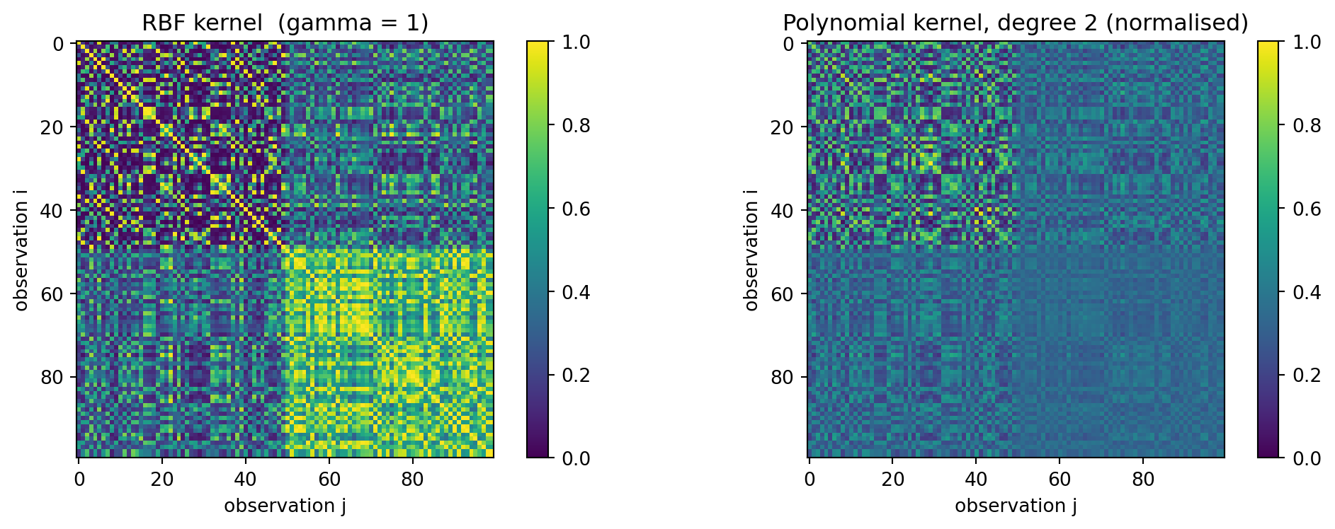

Figure 3: Kernel matrices for observations sorted by label.

4. The kernel SVM decision function

Replacing \(\mathbf{x}_i^\top\mathbf{x}_j\) with \(k(\mathbf{x}_i,\mathbf{x}_j)\) in the SVM dual gives the kernel SVM dual:

\[ \max_{\boldsymbol{\alpha}}\;\sum_{i=1}^{N}\alpha_i -\frac{1}{2}\sum_{i=1}^{N}\sum_{j=1}^{N} \alpha_i\alpha_j y_i y_j\,k(\mathbf{x}_i,\mathbf{x}_j) \qquad\text{subject to}\quad \alpha_i\geq 0,\quad\sum_{i=1}^{N}\alpha_i y_i=0. \]

The optimisation is entirely classical regardless of whether \(k\) is a classical formula or a quantum circuit.

At prediction time, the decision function is

\[ f(\mathbf{x}) =\operatorname{sign}\!\left(\sum_{i\in\mathcal{S}}\alpha_i y_i\,k(\mathbf{x}_i,\mathbf{x})+b\right), \]

where \(\mathcal{S}=\{i:\alpha_i>0\}\) is the support-vector index set. Only support vectors contribute to classifying a new observation.

configs = [
    ('linear', {},                        'Linear'),
    ('poly',   {'degree': 2, 'coef0': 1}, 'Polynomial  (degree 2)'),
    ('rbf',    {'gamma': 1.0},            'RBF  (gamma = 1)'),
]

fig, axes = plt.subplots(1, 3, figsize=(14, 4))
for ax, (kernel, params, title) in zip(axes, configs):
    clf = SVC(kernel=kernel, C=1.0, **params)
    clf.fit(X, y)
    Z = clf.predict(np.c_[xx.ravel(), yy.ravel()]).reshape(xx.shape)

    ax.contourf(xx, yy, Z, alpha=0.15, cmap='coolwarm')
    ax.contour(xx, yy, Z, colors='k', linewidths=0.8)
    for lbl, color in [(-1, '#3157a4'), (1, '#e07a3f')]:
        ax.scatter(*X[y == lbl].T, c=color, s=25)
    ax.scatter(
        *X[clf.support_].T,
        s=100, facecolors='none', edgecolors='k', linewidths=1.2,
    )
    acc = (clf.predict(X) == y).mean()
    ax.set_title(f'{title}\n{len(clf.support_)} SVs  |  train acc = {acc:.0%}', fontsize=9)
    ax.set(xlabel='$x_1$', ylabel='$x_2$', aspect='equal')

plt.tight_layout()
plt.show()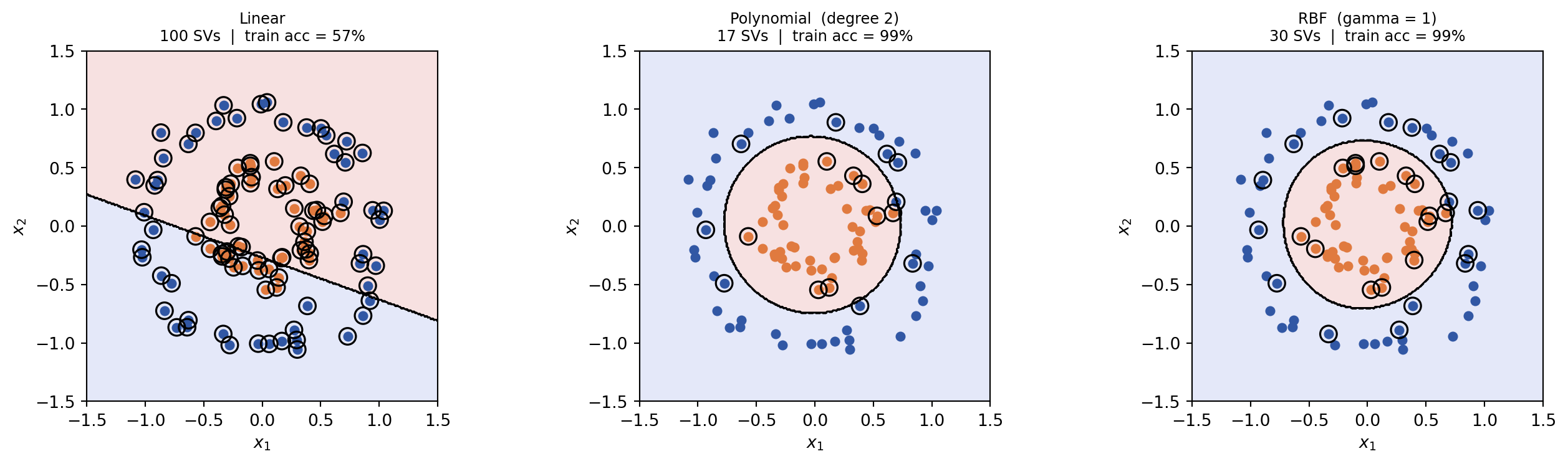

Figure 4: Decision boundaries produced by three different kernels on the concentric-ring dataset.

Try it yourself

Change RANDOM_SEED and rerun. Does the number of support vectors for each kernel stay roughly the same?
Increase noise in make_circles to 0.20. Which kernel degrades first?
Try gamma = 0.1 and gamma = 10 for the RBF kernel. How does the decision boundary change?
Add a sigmoid kernel to the comparison. What does the decision boundary look like?