%matplotlib inline
import matplotlib.pyplot as plt
import numpy as np
SVM Margin Geometry in Two Features
Derive the SVM constraint and margin width from three parallel lines in a two-feature space.
1. Line equation
A line in two-dimensional space can be written as
\[ x_2 = mx_1 + c, \]
where \(m\) is the slope and \(c\) is the intercept. In machine learning it is more convenient to use the inner-product form
\[ \vec{w}^\top\vec{x}+b=0, \qquad \vec{w}=\begin{pmatrix}w_1\\w_2\end{pmatrix},\quad \vec{x}=\begin{pmatrix}x_1\\x_2\end{pmatrix}. \]
Expanding the dot product gives \(w_1x_1+w_2x_2+b=0\). Putting \(x_2\) in terms of \(x_1\), the equation becomes
\[ x_2 = -\frac{w_1}{w_2}x_1 - \frac{b}{w_2}, \]
leading to a slope of \(-w_1/w_2\) and an intercept of \(-b/w_2\).
The vector \(\vec{w}\) is the normal to the line. To see why, take any two points \(\vec{x}^{(a)}\) and \(\vec{x}^{(b)}\) on the line. Both satisfy the line equation, so
\[ \vec{w}^\top\vec{x}^{(a)}+b=0,\qquad \vec{w}^\top\vec{x}^{(b)}+b=0. \]
Subtracting gives
\[ \vec{w}^\top(\vec{x}^{(a)}-\vec{x}^{(b)})=0. \]
The difference \(\vec{x}^{(a)}-\vec{x}^{(b)}\) is any vector that lies along the line, and its dot product with \(\vec{w}\) is zero, so \(\vec{w}\) is perpendicular to every direction along the line—that is, \(\vec{w}\) is the normal.
The next cell defines a line with \(\vec{w}=(1,1)^\top\) and \(b=-5\). We will further shift that line up and down by one unit and plot the three lines showing their equations on the plot.
from matplotlib.transforms import offset_copy

w = np.array([1.0, 1.0])
b = -5.0

x1 = np.linspace(0, 6, 300)
x2 = lambda c: (c - b - w[0] * x1) / w[1]

fig, ax = plt.subplots(figsize=(7, 6))
ax.plot(x1, x2(0), color='black', linewidth=2, label=r'$w_1x_1+w_2x_2+b=0$: $x_2=-x_1+5$')
ax.plot(x1, x2(1), '--', color='#e07a3f', label=r'$w_1x_1+w_2x_2+b=1$: $x_2=-x_1+6$')
ax.plot(x1, x2(-1), '--', color='#3157a4', label=r'$w_1x_1+w_2x_2+b=-1$: $x_2=-x_1+4$')

# Perpendicular margin arrow between the two support lines
ax.annotate('', xy=(3.5, 2.5), xytext=(2.5, 1.5),
            arrowprops=dict(arrowstyle='<->', color='green', lw=2))
# Shift label 45 display-pts upper-left (perpendicular to the arrow) from its midpoint
trans = offset_copy(ax.transData, fig=fig, x=-45, y=45, units='dots')
ax.text(3.0, 2.0, r'margin $=\frac{2}{\|\mathbf{w}\|}$', color='green',
        fontsize=10, rotation=45, ha='center', va='center', transform=trans)

ax.set(xlim=(0, 6), ylim=(0, 7), xlabel='$x_1$', ylabel='$x_2$',
    title=r'Three parallel lines for $\mathbf{w}=(1,1)^\top$, $b=-5$')
ax.set_aspect('equal')
ax.legend(loc='upper right')
ax.grid(alpha=0.2)

plt.show()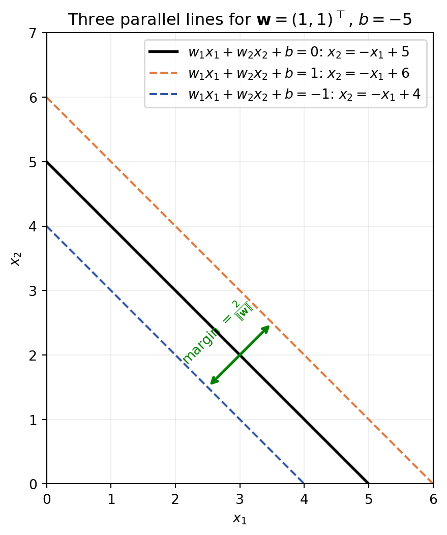
2. Geometric distance between parallel margin lines
Consider three parallel lines with normal vector \(\mathbf{w}=(1,1)^\top\) and offset \(b=-5\):
Central line: \(g(\mathbf{x})=\mathbf{w}^\top\mathbf{x}+b=0\), i.e. \(x_2=-x_1+5\);
Upper parallel line: \(g(\mathbf{x})=+1\), i.e. \(x_2=-x_1+6\);
Lower parallel line: \(g(\mathbf{x})=-1\), i.e. \(x_2=-x_1+4\).
All three lines are parallel because they have the same normal vector \(\mathbf{w}\) as derived earlier. Their common slope is \(-w_1/w_2=-1\), and they differ only in their intercepts.
The vector \(\mathbf{w}\) is perpendicular to all three lines. Therefore, the corresponding unit normal vector is \(\hat{\mathbf{n}}=\dfrac{\mathbf{w}}{\lVert\mathbf{w}\rVert}\) where \(\lVert\mathbf{w}\rVert=\sqrt{w_1^2+w_2^2}.\)
We now want to find the perpendicular distance between the two lines \(g(\mathbf{x})=+1\) and \(g(\mathbf{x})=-1\).
Let \(\mathbf{x}{-}\) be any point on the line \(g(\mathbf{x})=-1\). Moving from \(\mathbf{x}{-}\) in the direction of the unit normal until reaching the line \(g(\mathbf{x})=+1\) gives a point \(\mathbf{x}_{+}\). If \(D\) denotes the perpendicular distance between the two lines, then
\(\mathbf{x}{+}=\mathbf{x}{-}+D\dfrac{\mathbf{w}}{\lVert\mathbf{w}\rVert}\).
Since the two points lie on their respective lines, \(\mathbf{w}^\top\mathbf{x}_{+}+b=+1\) and \(\mathbf{w}^\top\mathbf{x}_{-}+b=-1\).
Subtracting the second equation from the first gives: \(2=\mathbf{w}^\top(\mathbf{x}{+}-\mathbf{x}{-})\).
Using \(\mathbf{x}{+}-\mathbf{x}{-}=D\dfrac{\mathbf{w}}{\lVert\mathbf{w}\rVert}\), we obtain: \(2=\mathbf{w}^\top\left(D\dfrac{\mathbf{w}}{\lVert\mathbf{w}\rVert}\right)\).
Therefore, \(2=D\dfrac{\mathbf{w}^\top\mathbf{w}}{\lVert\mathbf{w}\rVert}\). Since \(\mathbf{w}^\top\mathbf{w}=\lVert\mathbf{w}\rVert^2\),we get \(2=D\lVert\mathbf{w}\rVert\).
Hence, \(\boxed{D=\dfrac{2}{\lVert\mathbf{w}\rVert}}\).
The distance from the central line \(g(\mathbf{x})=0\) to either of the two parallel lines is therefore \(\boxed{\dfrac{1}{\lVert\mathbf{w}\rVert}}\).