Introduction Lead Publications Projects Math to Code Letters & Verse Light & Lens References Contact

Data Matrices, Variable Types, and Association

SD01 — Statistical Thinking

Course: Statistics and Probability for Data Science (DS14270).
Source deck: Samer El Kababji, SD01 — Statistical Thinking. Equations and teaching simulations below extend the deck’s concepts; they are not additional observations from the deck. Each file runs independently using base R, with knitr/R Markdown needed only for rendering.

Rows are observations; columns are variables

For \(n\) observations and \(p\) numeric variables, a data matrix has entries

\[ X=(x_{ij})\in\mathbb{R}^{n\times p},\qquad x_{ij}=\text{value of variable }j\text{ for observation }i. \]

Worked example — reading a matrix entry. With the three numeric columns used below, there are \(n=4\) rows and \(p=3\) columns, so \(X\) is a \(4\times3\) matrix. The entry \(x_{21}=25000\) is the loan amount in the second displayed record; \(x_{22}=9.43\) is that record’s interest rate.

An R data frame can also contain categorical columns. The next cell transcribes the four loan records visible in the deck (original row labels 1, 2, 3, 50). These are an excerpt, not the complete loan50 dataset or a random sample.

loans <- data.frame(
  loan_amount = c(7500, 25000, 14500, 3000),
  interest_rate = c(7.34, 9.43, 6.08, 7.96),
  term = c(36L, 60L, 36L, 36L),
  grade = ordered(c("A", "B", "A", "A"), levels = LETTERS[1:7]),
  state = factor(c("MD", "OH", "MO", "CA")),
  total_income = c(70000, 254000, 80000, 34000),
  homeownership = factor(c("rent", "mortgage", "mortgage", "rent")),
  row.names = c("1", "2", "3", "50")
)
loans

   loan_amount interest_rate term grade state total_income homeownership
1         7500          7.34   36     A    MD        70000          rent
2        25000          9.43   60     B    OH       254000      mortgage
3        14500          6.08   36     A    MO        80000      mortgage
50        3000          7.96   36     A    CA        34000          rent

loans["2", ]                 # one observational unit

  loan_amount interest_rate term grade state total_income homeownership
2       25000          9.43   60     B    OH       254000      mortgage

loans$term                   # one variable

[1] 36 60 36 36

X <- as.matrix(loans[c("loan_amount", "interest_rate", "total_income")])
dim(X)

[1] 4 3

X[2, 1]                      # x_21: second displayed record, first variable

[1] 25000

Do not convert the entire mixed-type data frame to a numeric matrix: factor codes would not represent meaningful amounts or distances.

Numeric, nominal, and ordinal variables

A discrete variable takes values in a countable set, such as a whole number of months. A continuous measurement is modeled on an interval of real numbers, even when recorded with rounding. Nominal categories have no inherent order; ordinal categories have an order without necessarily equal spacing.

\[ \text{Term}\in\{1,2,3,\ldots\},\qquad \text{Grade}\in\{A\prec B\prec\cdots\prec G\}. \]

Here \(\prec\) denotes category order, not a numerical gap. The statistical type of a variable is distinct from its R storage class.

data.frame(
  variable = names(loans),
  R_class = vapply(loans, function(z) paste(class(z), collapse = "/"), ""),
  statistical_type = c("numerical (amount)", "numerical (rate)",
                       "numerical discrete", "categorical ordinal",
                       "categorical nominal", "numerical (amount)",
                       "categorical nominal")
)

                   variable        R_class    statistical_type
loan_amount     loan_amount        numeric  numerical (amount)
interest_rate interest_rate        numeric    numerical (rate)
term                   term        integer  numerical discrete
grade                 grade ordered/factor categorical ordinal
state                 state         factor categorical nominal
total_income   total_income        numeric  numerical (amount)
homeownership homeownership         factor categorical nominal

is.ordered(loans$grade)

[1] TRUE

levels(loans$homeownership)

[1] "mortgage" "rent"    

Summarize a column according to its type

For numeric values, the sample mean is \(\bar x=n^{-1}\sum_i x_i\). For category \(c\), its relative frequency is \(\widehat p_c=n^{-1}\sum_i\mathbf{1}(x_i=c)\).

Worked examples using the four displayed records. For loan amount, the summation means adding the four amounts and dividing by four:

\[ \bar x=\frac{7500+25000+14500+3000}{4}=12500. \]

For just the category “rent”, the indicator \(\mathbf{1}(x_i=c)\) is 1 for a matching record and 0 otherwise:

\[ \widehat p_{\text{rent}}=\frac{1+0+0+1}{4}=0.5. \]

mean(loans$loan_amount)

[1] 12500

prop.table(table(loans$homeownership))

mortgage     rent 
     0.5      0.5 

These summarize only the four displayed records; they cannot characterize all borrowers or all 50 loans.

Association does not establish a causal link

For paired numeric variables, sample correlation is

\[ r=\frac{\sum_i(x_i-\bar x)(y_i-\bar y)} {\sqrt{\sum_i(x_i-\bar x)^2\sum_i(y_i-\bar y)^2}}. \]

Worked example — one small set of paired values. Suppose \(x=(1,2,3)\) and \(y=(2,4,3)\), so \(\bar x=2\) and \(\bar y=3\). The deviations are \((-1,0,1)\) and \((-1,1,0)\). Expanding each sum gives

\[ r=\frac{(-1)(-1)+(0)(1)+(1)(0)} {\sqrt{[(-1)^2+0^2+1^2][(-1)^2+1^2+0^2]}} =\frac{1}{\sqrt{2\times2}}=0.5. \]

The numerator adds paired deviation products; the denominator uses the sum of squared deviations for each variable.

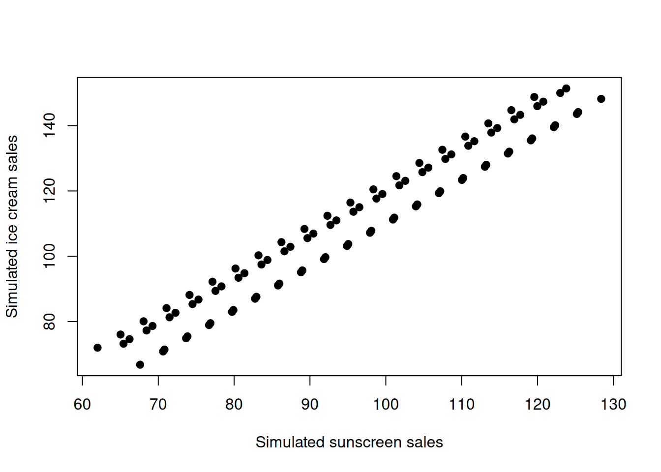
The deck’s sunscreen and ice cream example can arise from a shared cause: temperature. The following fictional sales include small day-to-day changes \(u\) and \(v\) in addition to the temperature effect:

\[ X=20+3T+u,\qquad Y=10+4T+v. \]

Worked example — substitute one day’s values. For \(T=20\), \(u=2\), and \(v=-4\):

\[ X=20+3(20)+2=82,\qquad Y=10+4(20)-4=86. \]

A warmer day raises both predicted sales through \(T\), even though neither formula contains the other sales variable.

Neither sales equation uses the other product’s sales.

set.seed(1101)
temperature <- seq(15, 35, length.out = 100)
sunscreen_variation <- rep(c(-3, 2, 0, 4, -2), length.out = 100)
ice_cream_variation <- rep(c(2, -4, 3, -1, 0), length.out = 100)
sunscreen <- 20 + 3 * temperature + sunscreen_variation
ice_cream <- 10 + 4 * temperature + ice_cream_variation
x_centered <- sunscreen - mean(sunscreen)
y_centered <- ice_cream - mean(ice_cream)
r_formula <- sum(x_centered * y_centered) /
  sqrt(sum(x_centered^2) * sum(y_centered^2))
c(formula = r_formula, R_correlation = cor(sunscreen, ice_cream))

      formula R_correlation 
    0.9754027     0.9754027 

plot(sunscreen, ice_cream, pch = 19,
     xlab = "Simulated sunscreen sales", ylab = "Simulated ice cream sales")

A strong correlation alone cannot tell us whether changing sunscreen sales would change ice cream sales. Also, zero correlation does not generally imply independence; correlation describes linear association.