Uniform Distribution and Monte Carlo Simulation

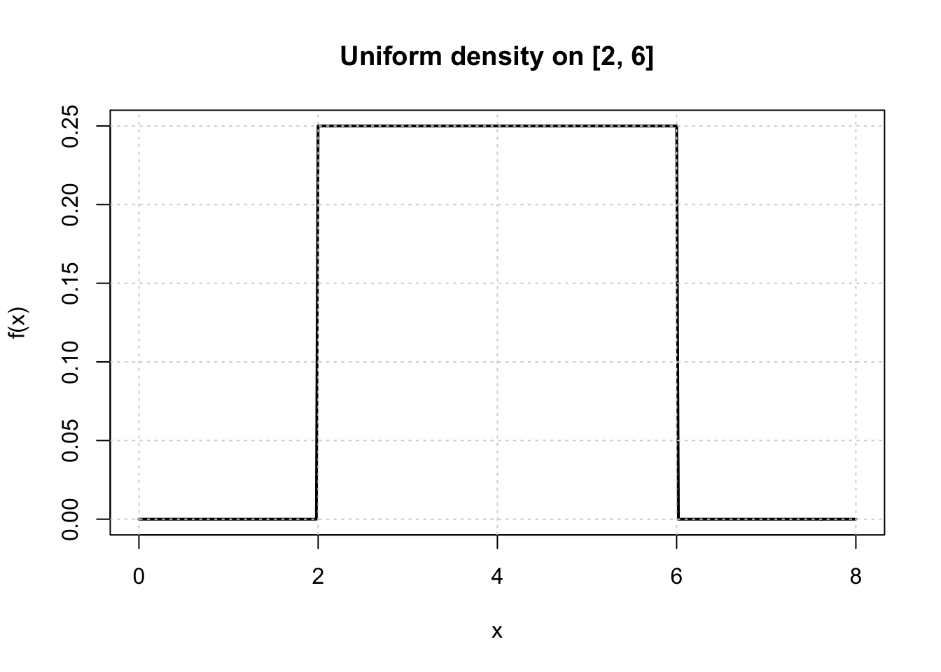
SD06 — Continuous Distributions

Author

Samer El Kababji

Course: Statistics and Probability for Data Science (DS14270).
Source deck: Samer El Kababji, SD06 — Continuous Distributions.

This lesson connects the continuous uniform distribution to simulation and Monte Carlo estimation. Computational experiments extend the deck and are labeled as such.

The continuous uniform distribution

For \(X\sim U(a,b)\), every equal-length subinterval inside \([a,b]\) has the same probability. Its density is

\[ f(x)= \begin{cases} \dfrac{1}{b-a}, & a\leq x\leq b,\\[4pt] 0, & \text{otherwise}. \end{cases} \]

Code

a <- 2
b <- 6
x <- seq(0, 8, length.out = 401)

plot(
  x, dunif(x, min = a, max = b), type = "l", lwd = 2,
  xlab = "x", ylab = "f(x)", main = "Uniform density on [2, 6]"
)
grid()

CDF and interval probabilities

Inside the support,

\[ F(x)=P(X\leq x)=\frac{x-a}{b-a}. \]

For \(a\leq c\leq d\leq b\),

\[ P(c\leq X\leq d)=\frac{d-c}{b-a}. \]

Thus, for \(X\sim U(2,6)\),

\[ P(3\leq X\leq5)=\frac{5-3}{6-2}=0.5. \]

Code

geometric_probability <- (5 - 3) / (6 - 2)
cdf_probability <- punif(5, 2, 6) - punif(3, 2, 6)

c(geometry = geometric_probability, R = cdf_probability)

geometry        R 
     0.5      0.5

For continuous variables, including or excluding endpoints does not change the probability because \(P(X=x)=0\).

Mean and variance

The center and spread are

\[ E(X)=\frac{a+b}{2},\qquad \operatorname{Var}(X)=\frac{(b-a)^2}{12}. \]

Code

a <- 2
b <- 6

c(
  mean = (a + b) / 2,
  variance = (b - a)^2 / 12,
  sd = (b - a) / sqrt(12)
)

    mean variance       sd 
4.000000 1.333333 1.154701

Random-number generation

runif() generates pseudorandom uniform values. The following is a fictional simulation extending the deck.

Code

set.seed(14270)
draws <- runif(100000, min = 2, max = 6)

c(
  simulated_mean = mean(draws),
  theoretical_mean = 4,
  simulated_variance = var(draws),
  theoretical_variance = 16 / 12,
  simulated_P_3_to_5 = mean(draws >= 3 & draws <= 5)
)

      simulated_mean     theoretical_mean   simulated_variance 
            3.991902             4.000000             1.333947 
theoretical_variance   simulated_P_3_to_5 
            1.333333             0.500150

Monte Carlo estimation of pi

Draw a point \((X,Y)\) uniformly from the square \([-1,1]^2\). The square has area 4, while the unit circle inside it has area \(\pi\). Therefore,

\[ P(X^2+Y^2\leq1)=\frac{\pi}{4} \]

and a Monte Carlo estimator is

\[ \widehat\pi=4\left(\frac{\text{points inside the circle}}{n}\right). \]

Code

set.seed(14270)
n <- 100000
x <- runif(n, -1, 1)
y <- runif(n, -1, 1)
inside <- x^2 + y^2 <= 1

pi_hat <- 4 * mean(inside)
c(estimate = pi_hat, truth = pi, error = pi_hat - pi)

     estimate         truth         error 
 3.1412800000  3.1415926536 -0.0003126536

Code

keep <- seq_len(2500)
plot(
  x[keep], y[keep], pch = 19, cex = 0.45,
  col = ifelse(inside[keep], "steelblue", "tomato"),
  asp = 1, xlab = "X", ylab = "Y", main = "Monte Carlo points"
)
symbols(0, 0, circles = 1, inches = FALSE, add = TRUE, lwd = 2)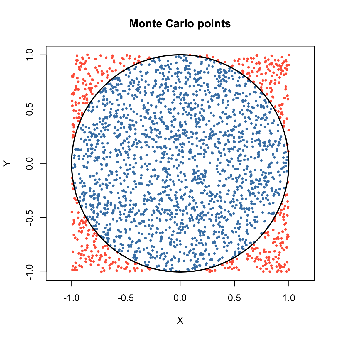

Practice questions

If \(X\sim U(10,18)\), find \(P(12\leq X\leq15)\).
Find \(E(X)\) and \(\operatorname{SD}(X)\).
Use qunif() to find the 90th percentile.
Why is the Monte Carlo estimate of \(\pi\) not exactly the same on every run unless the random seed is fixed?

Check your answers

The probability is \((15-12)/(18-10)=3/8=0.375\).
The mean is 14 and the standard deviation is \(8/\sqrt{12}\approx2.309\).
qunif(0.90, 10, 18) gives \(17.2\).
It is computed from a finite random sample, so the sampled proportion has simulation variability.