Weibull Distribution and Survival

SD06 — Continuous Distributions

Author

Samer El Kababji

Course: Statistics and Probability for Data Science (DS14270).
Source deck: Samer El Kababji, SD06 — Continuous Distributions.

The Weibull distribution is a flexible model for lifetimes and survival. In this lesson, \(k\) is the shape and \(\lambda\) is the scale, matching the deck and base R.

Density, CDF, and survival function

For \(X\sim\operatorname{Weibull}(k,\lambda)\),

\[ f(x)=\frac{k}{\lambda} \left(\frac{x}{\lambda}\right)^{k-1} \exp\left[-\left(\frac{x}{\lambda}\right)^k\right], \qquad x\geq0, \]

and

\[ F(x)=1-\exp\left[-\left(\frac{x}{\lambda}\right)^k\right]. \]

Therefore the survival function is

\[ S(x)=P(X>x)=\exp\left[-\left(\frac{x}{\lambda}\right)^k\right]. \]

Code

shape <- 2
scale <- 100
x <- c(0, 40, 80, 120)

data.frame(
  x,
  density = dweibull(x, shape = shape, scale = scale),
  CDF = pweibull(x, shape = shape, scale = scale),
  survival = pweibull(
    x, shape = shape, scale = scale, lower.tail = FALSE
  )
)

    x     density       CDF  survival
1   0 0.000000000 0.0000000 1.0000000
2  40 0.006817150 0.1478562 0.8521438
3  80 0.008436679 0.4727076 0.5272924
4 120 0.005686266 0.7630722 0.2369278

Component-lifetime example

For shape \(k=2\) and scale \(\lambda=100\),

\[ P(X<80)=1-\exp[-(80/100)^2]\approx0.4727. \]

Code

c(
  formula = 1 - exp(-(80 / 100)^2),
  R = pweibull(80, shape = 2, scale = 100)
)

  formula         R 
0.4727076 0.4727076

Mean and variance

The moments use the gamma function:

\[ E(X)=\lambda\Gamma\left(1+\frac1k\right), \]

\[ \operatorname{Var}(X)=\lambda^2\left[ \Gamma\left(1+\frac2k\right)- \Gamma\left(1+\frac1k\right)^2 \right]. \]

Code

k <- 2
lambda <- 100

mu <- lambda * gamma(1 + 1 / k)
variance <- lambda^2 * (
  gamma(1 + 2 / k) - gamma(1 + 1 / k)^2
)

c(mean = mu, variance = variance, sd = sqrt(variance))

      mean   variance         sd 
  88.62269 2146.01837   46.32514

Shape and failure behavior

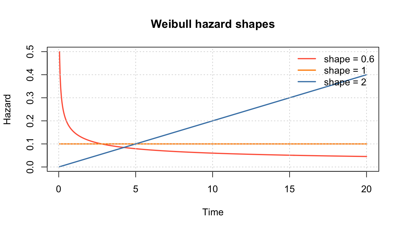
The Weibull hazard function is

\[ h(x)=\frac{f(x)}{S(x)} =\frac{k}{\lambda}\left(\frac{x}{\lambda}\right)^{k-1}. \]

\(k<1\): decreasing hazard, often associated with early failures.
\(k=1\): constant hazard; the Weibull becomes exponential.
\(k>1\): increasing hazard, often associated with wear-out.

Code

x <- seq(0.05, 20, length.out = 500)
shapes <- c(0.6, 1, 2)
colors <- c("tomato", "darkorange", "steelblue")

matplot(
  x,
  sapply(shapes, function(k) (k / 10) * (x / 10)^(k - 1)),
  type = "l", lty = 1, lwd = 2, col = colors,
  xlab = "Time", ylab = "Hazard", main = "Weibull hazard shapes"
)
legend("topright", legend = paste("shape =", shapes), col = colors,
       lty = 1, lwd = 2, bty = "n")
grid()

Scale changes the time axis

For fixed shape, a larger scale stretches lifetimes. Because

\[ F(\lambda)=1-e^{-1}\approx0.632, \]

the scale is the time by which about 63.2% of the population has experienced the event.

The deck’s survival context uses shape 2 and scale 12 months.

Code

times <- c(6, 12, 18, 24)
data.frame(
  months = times,
  survival_probability = pweibull(
    times, shape = 2, scale = 12, lower.tail = FALSE
  )
)

  months survival_probability
1      6           0.77880078
2     12           0.36787944
3     18           0.10539922
4     24           0.01831564

These are model-based probabilities, not patient predictions.

Practice questions

For shape 1.5 and scale 20, find \(P(X\leq10)\).
Find \(P(X>25)\).
Is the hazard increasing or decreasing?
What special distribution results when the shape is 1?

Check your answers

pweibull(10, 1.5, 20) gives approximately \(0.2978\).
pweibull(25, 1.5, 20, lower.tail = FALSE) gives approximately \(0.2472\).
It is increasing because \(k=1.5>1\).
An exponential distribution with rate \(1/\lambda\).