Course: Statistics and Probability for Data Science (DS14270).
Source deck: Samer El Kababji, SD06 — Continuous Distributions.
This lesson covers the normal density, standardization, probability calculations, the empirical rule, and linear combinations of normal variables.
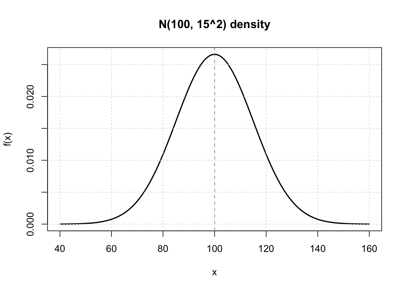
The normal model
If \(X\sim N(\mu,\sigma^2)\), then
\[
f(x)=\frac{1}{\sigma\sqrt{2\pi}}
\exp\left[-\frac{(x-\mu)^2}{2\sigma^2}\right],
\qquad -\infty<x<\infty.
\]
Its mean is \(\mu\) and its variance is \(\sigma^2\).
Code
mu <- 100
sigma <- 15
x <- seq(mu - 4 * sigma, mu + 4 * sigma, length.out = 501)

plot(
  x, dnorm(x, mean = mu, sd = sigma), type = "l", lwd = 2,
  xlab = "x", ylab = "f(x)", main = "N(100, 15^2) density"
)
abline(v = mu, lty = 2, col = "steelblue")
grid()
The standard normal variable \(Z\sim N(0,1)\) has density \(\phi(z)\) and CDF \(\Phi(z)=P(Z\leq z)\).
Z-scores
Standardization converts a normal variable to the standard normal scale:
\[
Z=\frac{X-\mu}{\sigma}.
\]
A z-score tells how many standard deviations a value lies above or below the mean. With exam mean 70, standard deviation 10, and score 85,
\[
z=\frac{85-70}{10}=1.5.
\]
Code
score <- 85
mu <- 70
sigma <- 10
z <- (score - mu) / sigma
z
Probability by standardization
For any cutoff \(x\),
\[
P(X\leq x)=P\left(Z\leq\frac{x-\mu}{\sigma}\right).
\]
In the deck, \(X\sim N(100,15^2)\). For \(x=120\),
\[
z=\frac{120-100}{15}\approx1.33,
\]
so \(P(X\leq120)\approx0.9082\) when a z-table rounds to 1.33. R retains the unrounded z-score.
Code
z_exact <- (120 - 100) / 15
c(
  exact_z_in_R = pnorm(z_exact),
  rounded_z_table = pnorm(1.33),
  direct = pnorm(120, mean = 100, sd = 15)
)
   exact_z_in_R rounded_z_table          direct
      0.9087888       0.9082409       0.9087888
The 68–95–99.7 rule
For a normal distribution, approximately 68%, 95%, and 99.7% of observations fall within 1, 2, and 3 standard deviations of the mean.
Code
k <- 1:3
exact_probabilities <- pnorm(k) - pnorm(-k)

data.frame(
  interval = paste0("mu +/- ", k, " sigma"),
  exact_probability = exact_probabilities,
  rule_of_thumb = c(0.68, 0.95, 0.997)
)
        interval exact_probability rule_of_thumb
1 mu +/- 1 sigma         0.6826895         0.680
2 mu +/- 2 sigma         0.9544997         0.950
3 mu +/- 3 sigma         0.9973002         0.997
Quantiles
The \(p\)th quantile satisfies \(P(X\leq x_p)=p\) and is
\[
x_p=\mu+\sigma z_p,
\qquad z_p=\Phi^{-1}(p).
\]
Code
p <- c(0.025, 0.50, 0.975)
data.frame(
  probability = p,
  standard_normal = qnorm(p),
  N_100_15_squared = qnorm(p, mean = 100, sd = 15)
)
  probability standard_normal N_100_15_squared
1       0.025       -1.959964         70.60054
2       0.500        0.000000        100.00000
3       0.975        1.959964        129.39946
Practice questions
- If \(X\sim N(50,8^2)\), find the z-score of 62.
- Find \(P(X\leq62)\) and \(P(42\leq X\leq58)\).
- Find the 90th percentile of \(X\).
- If independent \(X\sim N(10,3^2)\) and \(Y\sim N(4,2^2)\), give the distribution of \(X-Y\).
- \(z=(62-50)/8=1.5\).
pnorm(62, 50, 8) is approximately \(0.9332\); the central interval has probability pnorm(58, 50, 8) - pnorm(42, 50, 8), approximately \(0.6827\).qnorm(0.90, 50, 8) is approximately \(60.25\).- \(X-Y\sim N(6,13)\) because means subtract but independent variances add.