Code
interest_rate <- rep(
  c(5, 6, 7, 8, 9, 10, 11, 12, 13, 14, 16, 18, 20, 25, 27),
  times = c(3, 4, 6, 8, 8, 6, 3, 3, 2, 2, 1, 1, 1, 1, 1)
)
stopifnot(length(interest_rate) == 50)
SD02 — Exploratory Data Analysis
Course: Statistics and Probability for Data Science (DS14270).
Source deck: Samer El Kababji, SD02 — Exploratory Data Analysis.
This lesson uses a fictional set of 50 interest rates. The values were chosen to demonstrate exploratory plots and are not the loan50 observations shown in the deck.
interest_rate <- rep(
c(5, 6, 7, 8, 9, 10, 11, 12, 13, 14, 16, 18, 20, 25, 27),
times = c(3, 4, 6, 8, 8, 6, 3, 3, 2, 2, 1, 1, 1, 1, 1)
)
stopifnot(length(interest_rate) == 50)A dot plot places one dot at each observed value. Repeated values can be stacked, so the stack height represents frequency.
For value \(a\), its frequency is
\[ f(a)=\sum_{i=1}^{n}\mathbf{1}(x_i=a). \]
Worked example — count a matching value. For a tiny dataset \((5,6,6,8)\) and \(a=6\), the indicators are \((0,1,1,0)\):
\[ f(6)=0+1+1+0=2. \]
Two dots therefore stack at 6.
frequencies <- table(interest_rate)
frequencies
interest_rate
5 6 7 8 9 10 11 12 13 14 16 18 20 25 27
3 4 6 8 8 6 3 3 2 2 1 1 1 1 1 stripchart(interest_rate, method = "stack", pch = 19,
col = "steelblue", offset = 0.6,
xlab = "Interest rate (%)",
main = "Stacked dot plot of fictional interest rates")
abline(v = mean(interest_rate), col = "tomato", lwd = 2, lty = 2)
legend("topright", "Mean", col = "tomato", lwd = 2, lty = 2,
bty = "n")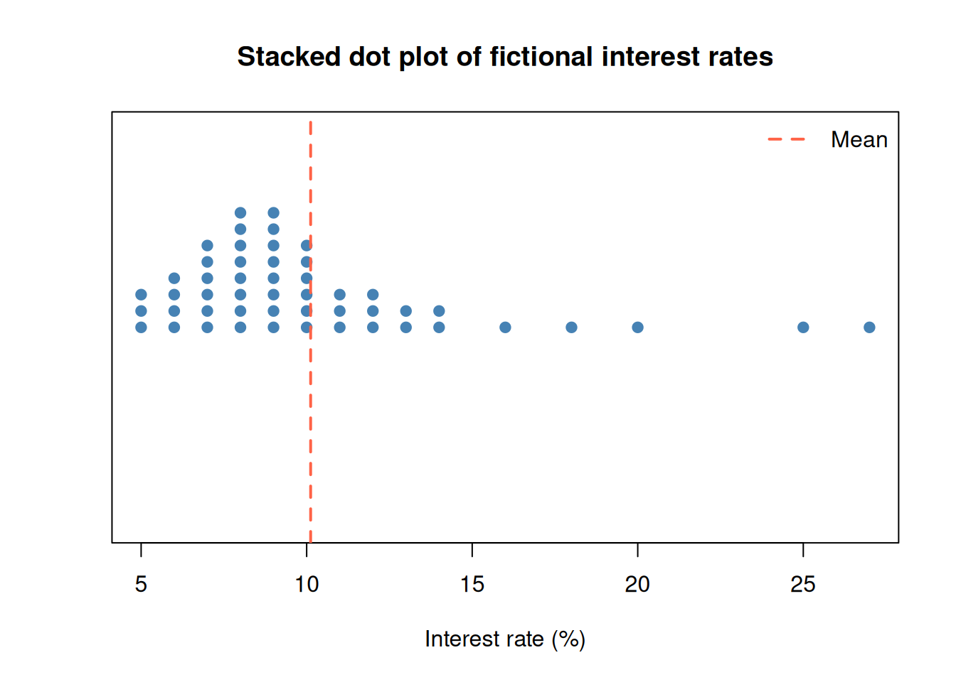
Rounding makes stacking easier to see, but it removes detail. The displayed shape can therefore depend on measurement precision.
A histogram divides the number line into intervals called bins. For bin \(B_k\), its frequency is
\[ f_k=\sum_{i=1}^{n}\mathbf{1}(x_i\in B_k). \]
Worked example — count values in a bin. For \((5,6,6,8)\), take the bin \(B_k=[6,8)\): include 6 but exclude 8. Then
\[ f_k=0+1+1+0=2. \]
The value 8 goes into the next bin. This matches right = FALSE below.
hist(interest_rate, breaks = seq(4, 28, by = 2), right = FALSE,
     col = "steelblue", border = "white",
     xlab = "Interest rate (%)", ylab = "Frequency",
     main = "Histogram of fictional interest rates")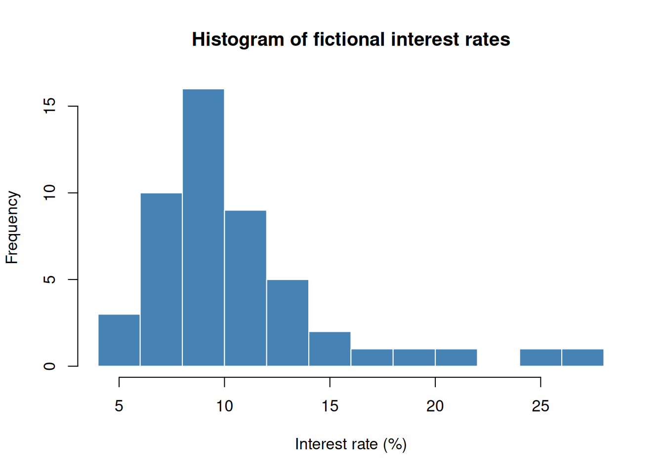
Changing the bin boundaries can change the appearance. Explore several reasonable choices before describing peaks or gaps.
The fictional data have a long right tail. A few large observations pull the mean farther right than the median.
c(mean = mean(interest_rate), median = median(interest_rate)) mean median
10.12 9.00 Using the sample standard deviation \(s\), the standardized value is
\[ z_i=\frac{x_i-\bar{x}}{s}. \]
Worked example — standardize a small dataset. Take \(x=(1,1,4)\). Its mean is \(\bar{x}=2\) and its sample variance is \([(-1)^2+(-1)^2+2^2]/(3-1)=3\), giving \(s=\sqrt{3}\):
\[ z_1=z_2=\frac{1-2}{\sqrt{3}}\approx-0.57735,\qquad z_3=\frac{4-2}{\sqrt{3}}\approx1.15470. \]
The last observation is about 1.15 sample standard deviations above the mean.
The skewness formula used in the deck is the average cubed standardized value:
\[ g_1=\frac{1}{n}\sum_{i=1}^{n}z_i^3. \]
Worked example — cube, add, and average. Using the same three standardized values, keep the exact fractions until the last step:
\[ g_1=\frac{(-1/\sqrt{3})^3+(-1/\sqrt{3})^3+(2/\sqrt{3})^3}{3} =\frac{2}{3\sqrt{3}}\approx0.38490. \]
The positive result reflects the longer right tail of \((1,1,4)\).
Negative values suggest a longer left tail, values near zero suggest a roughly symmetric shape, and positive values suggest a longer right tail.
n <- length(interest_rate)
x_bar <- mean(interest_rate)
s <- sd(interest_rate)
z <- (interest_rate - x_bar) / s
g1 <- mean(z^3)
g1
[1] 1.918931Using the same standardized values, the kurtosis formula in the deck is
\[ g_2=\frac{1}{n}\sum_{i=1}^{n}z_i^4. \]
Worked example — fourth powers of the same values. For \(x=(1,1,4)\),
\[ g_2=\frac{(-1/\sqrt{3})^4+(-1/\sqrt{3})^4+(2/\sqrt{3})^4}{3} =\frac{1/9+1/9+16/9}{3}=\frac{2}{3}\approx0.66667. \]
Under this lesson’s convention, excess kurtosis is \(g_2-3=2/3-3=-7/3\approx-2.33333\). This tiny example illustrates the arithmetic; it is too small to support a reliable description of population tails.
Large fourth powers give unusual observations in the tails substantial weight.
g2 <- mean(z^4)
c(skewness = g1, kurtosis = g2)
skewness kurtosis
1.918931 7.014032 Kurtosis is often compared with 3, while some software instead reports excess kurtosis, \(g_2-3\). Software may also apply small-sample corrections, so the formula and convention should accompany the reported value.
A prominent peak is called a mode. A shape may be described as unimodal, bimodal, or multimodal according to the number of prominent peaks. These constructed values let us compare those patterns without assuming any probability model.
unimodal <- rep(1:9, times = c(1, 3, 6, 10, 14, 10, 6, 3, 1))
bimodal <- c(
  rep(1:7, times = c(1, 4, 9, 5, 2, 1, 1)),
  rep(12:18, times = c(1, 1, 2, 5, 9, 4, 1))
)
multimodal <- c(
  rep(1:5, times = c(2, 7, 10, 5, 2)),
  rep(8:12, times = c(2, 7, 10, 5, 2)),
  rep(15:19, times = c(2, 7, 10, 5, 2))
)

old_mfrow <- par("mfrow")
par(mfrow = c(1, 3))
hist(unimodal, breaks = seq(0.5, 19.5, by = 1),
     col = "steelblue", main = "Unimodal", xlab = "Value")
hist(bimodal, breaks = seq(0.5, 19.5, by = 1),
     col = "steelblue", main = "Bimodal", xlab = "Value")
hist(multimodal, breaks = seq(0.5, 19.5, by = 1),
     col = "steelblue", main = "Multimodal", xlab = "Value")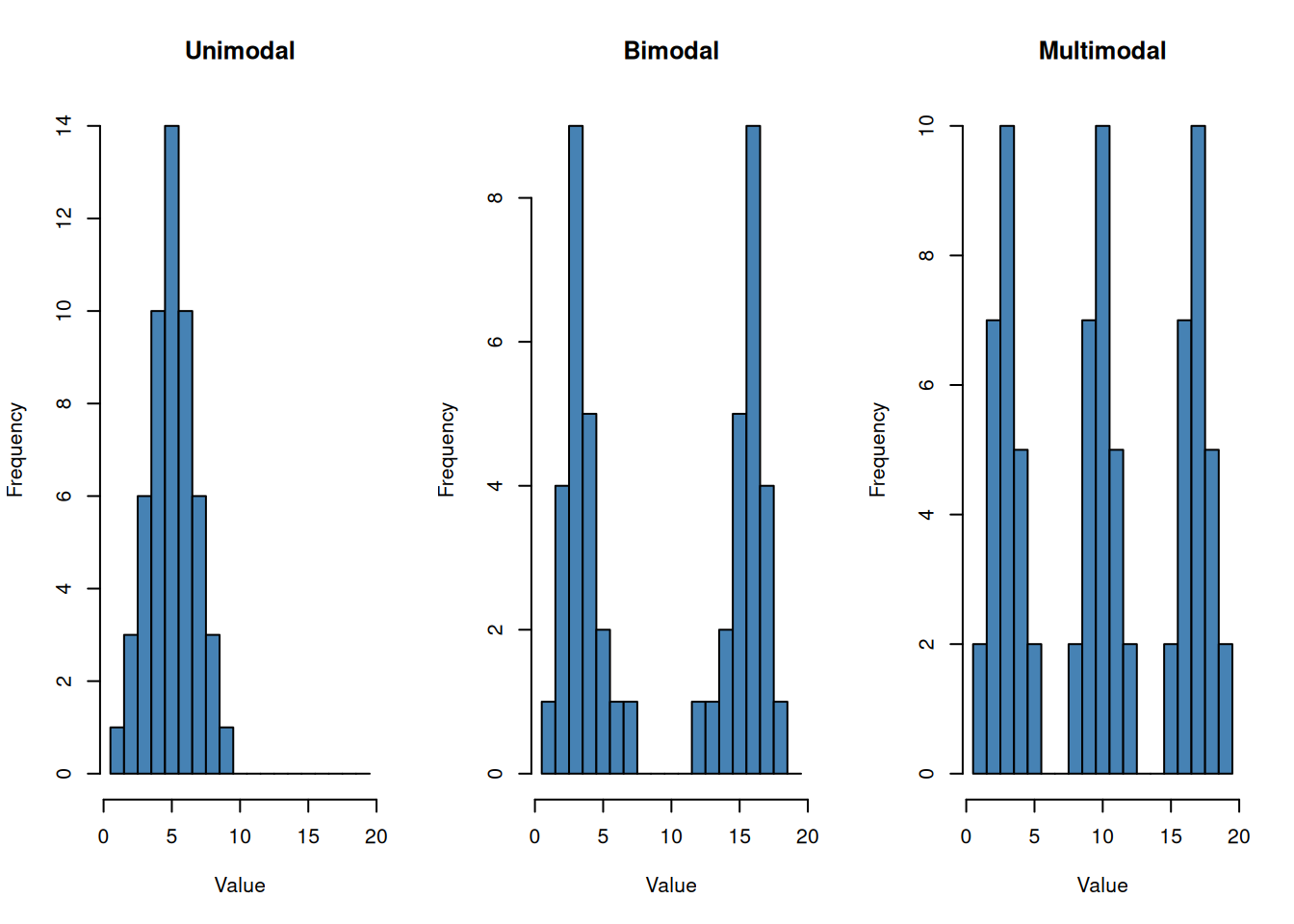
par(mfrow = old_mfrow)The number of apparent peaks can change with histogram bins. Focus on prominent, stable features rather than every small fluctuation.
The interquartile range is the distance between the third and first quartiles:
\[ IQR=Q_3-Q_1. \]
The usual outlier fences are
\[ \text{lower fence}=Q_1-1.5(IQR),\qquad \text{upper fence}=Q_3+1.5(IQR). \]
Worked example — calculate the fences. For the six ordered values \((3,5,8,9,14,21)\), the type = 7 quartiles are \(Q_1=5.75\) and \(Q_3=12.75\):
\[ IQR=12.75-5.75=7, \]
\[ \text{lower fence}=5.75-1.5(7)=-4.75,\qquad \text{upper fence}=12.75+1.5(7)=23.25. \]
All six observations lie within these fences. The whiskers reach the observed values 3 and 21, rather than the fence positions. A new observation at 30 would exceed these fixed fences; adding it to the dataset would require recalculating the quartiles and fences.
Values beyond the fences are shown separately as suspected outliers. A value flagged by this rule is not automatically an error.
quartiles <- quantile(interest_rate, c(0.25, 0.50, 0.75), type = 7)
q1 <- unname(quartiles[1])
median_x <- unname(quartiles[2])
q3 <- unname(quartiles[3])
iqr <- q3 - q1
lower_fence <- q1 - 1.5 * iqr
upper_fence <- q3 + 1.5 * iqr

lower_whisker <- min(interest_rate[interest_rate >= lower_fence])
upper_whisker <- max(interest_rate[interest_rate <= upper_fence])
suspected_outliers <- interest_rate[
  interest_rate < lower_fence | interest_rate > upper_fence
]

c(Q1 = q1, median = median_x, Q3 = q3, IQR = iqr,
  lower_fence = lower_fence, upper_fence = upper_fence,
  lower_whisker = lower_whisker, upper_whisker = upper_whisker)
Q1 median Q3 IQR lower_fence
7.250 9.000 11.000 3.750 1.625
upper_fence lower_whisker upper_whisker
16.625 5.000 16.000 suspected_outliers[1] 18 20 25 27The next cell draws a box plot directly from these type = 7 calculations.
x_limits <- range(c(interest_rate, lower_whisker, upper_whisker))
plot(NA, xlim = x_limits, ylim = c(0.5, 1.5), yaxt = "n",
     xlab = "Interest rate (%)", ylab = "",
     main = "Box plot of fictional interest rates")
rect(q1, 0.8, q3, 1.2, col = "lightblue")
segments(median_x, 0.8, median_x, 1.2, lwd = 3)
segments(lower_whisker, 1, q1, 1)
segments(q3, 1, upper_whisker, 1)
segments(lower_whisker, 0.9, lower_whisker, 1.1)
segments(upper_whisker, 0.9, upper_whisker, 1.1)
points(suspected_outliers, rep(1, length(suspected_outliers)),
       pch = 19, col = "tomato")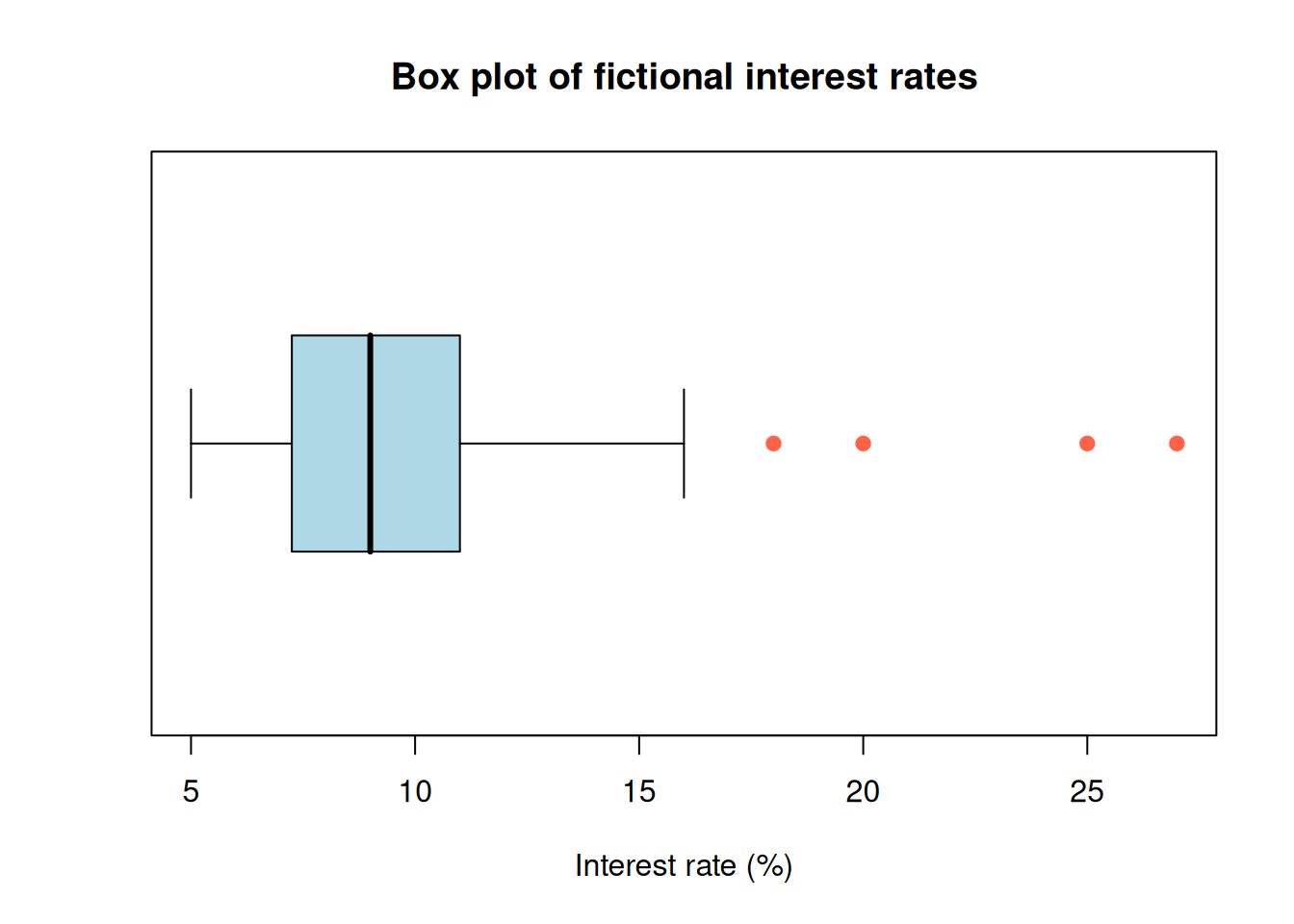
Try it: remove the values 25 and 27, then recompute the mean, median, skewness, kurtosis, and outlier fences. Which summaries change most?