Course: Statistics and Probability for Data Science (DS14270). Source deck: Samer El Kababji, SD01 — Statistical Thinking. Equations and teaching simulations below extend the deck’s concepts; they are not additional observations from the deck. Each file runs independently using base R, with knitr/R Markdown needed only for rendering.
Define the population and its target quantity
A sample is a subset of a population. The drug question in the deck targets people with severe heart disease; it is not restricted to the one anecdotal patient. For a computational sampling example, use a fictional league of players, where teams are groups and salary is measured in thousands of dollars. No real league salaries are used.
For a finite population of size \(N\), its mean is
\[
\mu=\frac{1}{N}\sum_{i=1}^N y_i.
\]
Worked example — a tiny fictional population. If the entire population has four salaries \(y=(60,70,80,90)\) (in thousands of dollars), then
\[
\mu=\frac{60+70+80+90}{4}=75.
\]
The sum adds every population value. The simulation below uses a larger fictional population.
Worked example — one sample. From the four-player illustration above, suppose the selected salaries are 60 and 80. The sum includes only these sampled players:
\[
\bar y=\frac{60+80}{2}=70.
\]
One sample mean can differ from \(\mu=75\); \(E(\bar y)=\mu\) describes the average over all possible simple random samples.
Code
n <-80srs <- population[sample.int(N, n, replace =FALSE), ]c(sample_size =nrow(srs), sample_mean =mean(srs$salary), population_mean = mu)
Worked example — one stratified estimate. In a separate small example, suppose two teams contain 40 and 60 players, with sampled mean salaries of 70 and 90. Expand the sum into one weighted term per team:
With equal team sizes and eight sampled per team, the ordinary sample mean also equals the weighted mean. With unequal team sizes and equal allocation, use the population weights rather than averaging strata equally.
Cluster sampling: include everyone in selected clusters
Now treat team as a cluster. Select \(m\) teams from \(H\) teams and include all players on those teams. Each person’s inclusion probability is \(m/H\). For known population size \(N\), a design-unbiased estimator is
Worked example — one selected cluster. In a separate tiny league with \(H=3\) teams of two players each, \(N=6\). Suppose \(m=1\) team is selected, and its two salaries are 60 and 80. The inner sum adds salaries within that team; the outer sum has only one selected team:
Equal cluster sizes make this estimator equal to the sample mean here. Players on one team share a salary component, so 80 clustered observations need not contain as much information as 80 simple-random-sample observations. The SRS standard-error formula above does not apply to this clustered design.
Multistage sampling: sample within selected clusters
Select \(m\) teams, then select \(k\) players from each selected team of size \(N_h\). The person’s inclusion probability and an inverse-probability estimator are
Worked example — one selected team. Use the tiny six-player league above, but now sample \(k=1\) player from the selected team of size \(N_h=2\). If that player’s salary is 80, then
Here both sums have one term. Dividing the observed salary by its inclusion probability gives its estimated contribution to the population total, which is then divided by \(N\). The code below uses the larger simulated league.
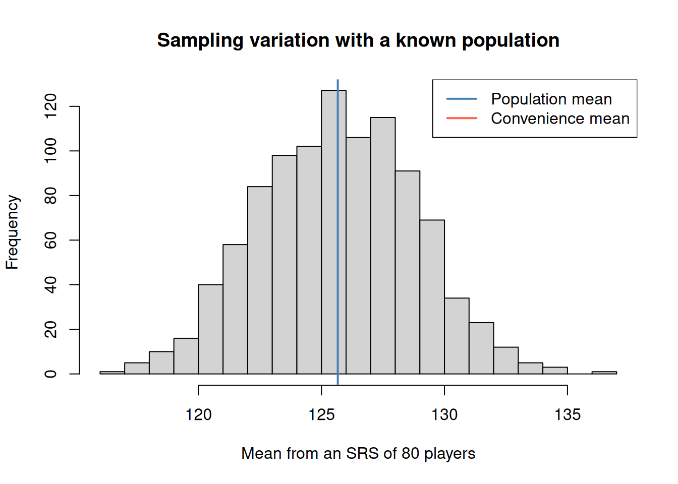
Taking players only from the first two teams gives zero inclusion probability to everyone else. Repeating that procedure cannot remove its systematic bias. For comparison, repeated SRS estimates fluctuate around the population mean:
Worked example — average over all possible samples. Suppose a tiny population has mean \(\mu=10\), and a sampling procedure has two equally likely possible samples whose estimates are 11 and 13. Then
hist(repeated_srs, breaks =25, xlab ="Mean from an SRS of 80 players",main ="Sampling variation with a known population")abline(v = mu, col ="steelblue", lwd =2)abline(v =mean(convenience$salary), col ="tomato", lwd =2)legend("topright", c("Population mean", "Convenience mean"),col =c("steelblue", "tomato"), lwd =2)
Random selection reduces selection bias under the sampling design, but nonresponse or incomplete population coverage can still bias the final data.
Try it: select only one cluster. Explain why its mean can differ greatly from the population mean even though the cluster was selected randomly.