Joint Random Variables, Covariance, and Correlation

SD04 — Random Variables

Author

Samer El Kababji

Course: Statistics and Probability for Data Science (DS14270).
Source deck: Samer El Kababji, SD04 — Random Variables.

This lesson develops the deck’s joint-distribution example, derives marginal distributions, covariance, and correlation, and clarifies how zero covariance differs from independence. The practice questions and computational examples extend the deck’s concepts.

Joint and marginal distributions

For discrete random variables \(X\) and \(Y\), the joint PMF is

\[ p_{X,Y}(x,y)=P(X=x,Y=y). \]

A valid joint PMF satisfies

\[ p_{X,Y}(x,y)\geq0, \qquad \sum_x\sum_y p_{X,Y}(x,y)=1. \]

Summing across the other variable produces a marginal PMF:

\[ p_X(x)=\sum_y p_{X,Y}(x,y), \qquad p_Y(y)=\sum_x p_{X,Y}(x,y). \]

Worked example: a joint probability table

The deck uses \(X\in\{1,3\}\) and \(Y\in\{2,4\}\) with joint probabilities

\(X\backslash Y\) 2 4 \(p_X(x)\)
1 0.2 0.3 0.5
3 0.1 0.4 0.5
\(p_Y(y)\) 0.3 0.7 1.0

For example,

\[ P(X=1,Y=2)=0.2. \]

The row and column sums give

\[ p_X(1)=0.5,\quad p_X(3)=0.5, \qquad p_Y(2)=0.3,\quad p_Y(4)=0.7. \]

Code
x_values <- c(1, 3)
y_values <- c(2, 4)

joint_pmf <- matrix(
  c(0.2, 0.3,
    0.1, 0.4),
  nrow = 2,
  byrow = TRUE,
  dimnames = list(X = x_values, Y = y_values)
)

p_X <- rowSums(joint_pmf)
p_Y <- colSums(joint_pmf)

joint_pmf
   Y
X     2   4
  1 0.2 0.3
  3 0.1 0.4
Code
p_X
  1   3 
0.5 0.5 
Code
p_Y
  2   4 
0.3 0.7 
Code
stopifnot(isTRUE(all.equal(sum(joint_pmf), 1)))

Expectations from a joint PMF

Marginal distributions are sufficient for the individual means:

\[ E(X)=\sum_x x p_X(x) =1(0.5)+3(0.5)=2, \]

\[ E(Y)=\sum_y y p_Y(y) =2(0.3)+4(0.7)=3.4. \]

The product moment uses the joint distribution:

\[ \begin{aligned} E(XY) &=\sum_x\sum_y xy\,p_{X,Y}(x,y)\\ &=2(0.2)+4(0.3)+6(0.1)+12(0.4)\\ &=7. \end{aligned} \]

Code
joint_grid <- expand.grid(X = x_values, Y = y_values)
joint_grid$probability <- as.vector(joint_pmf)
joint_grid$XY <- with(joint_grid, X * Y)

E_X <- sum(x_values * p_X)
E_Y <- sum(y_values * p_Y)
E_XY <- with(joint_grid, sum(XY * probability))

joint_grid
  X Y probability XY
1 1 2         0.2  2
2 3 2         0.1  6
3 1 4         0.3  4
4 3 4         0.4 12
Code
c(E_X = E_X, E_Y = E_Y, E_XY = E_XY)
 E_X  E_Y E_XY 
 2.0  3.4  7.0 

R matrices are stored column by column. expand.grid() changes its first column fastest, so as.vector(joint_pmf) aligns the four joint probabilities with the displayed \((X,Y)\) pairs.

Covariance

Covariance measures whether deviations from the two means tend to have the same sign or opposite signs:

\[ \operatorname{Cov}(X,Y) =E\bigl[(X-E(X))(Y-E(Y))\bigr]. \]

Expanding the product gives the computational identity

\[ \operatorname{Cov}(X,Y)=E(XY)-E(X)E(Y). \]

For the joint table,

\[ \operatorname{Cov}(X,Y)=7-(2)(3.4)=0.2. \]

Code
covariance_centered <- with(
  joint_grid,
  sum((X - E_X) * (Y - E_Y) * probability)
)
covariance_moments <- E_XY - E_X * E_Y

c(
  centered_definition = covariance_centered,
  moment_identity = covariance_moments
)
centered_definition     moment_identity 
                0.2                 0.2 
Code
stopifnot(isTRUE(all.equal(covariance_centered,
                           covariance_moments)))

Covariance depends on measurement units. If \(X\) is multiplied by \(a\) and \(Y\) by \(b\), then

\[ \operatorname{Cov}(aX+c,bY+d) =ab\operatorname{Cov}(X,Y). \]

Code
a <- 100
b <- -2

transformed_covariance <- with(
  joint_grid,
  sum(
    ((a * X + 5) - (a * E_X + 5)) *
    ((b * Y - 10) - (b * E_Y - 10)) *
    probability
  )
)

c(
  transformed_direct = transformed_covariance,
  transformed_rule = a * b * covariance_moments
)
transformed_direct   transformed_rule 
               -40                -40 

Independence and covariance

Discrete \(X\) and \(Y\) are independent when the joint PMF factors at every pair:

\[ p_{X,Y}(x,y)=p_X(x)p_Y(y) \quad\text{for every }x,y. \]

The example is not independent. At \((1,2)\),

\[ p_{X,Y}(1,2)=0.2 \neq p_X(1)p_Y(2)=(0.5)(0.3)=0.15. \]

Code
pmf_if_independent <- outer(p_X, p_Y)
dimnames(pmf_if_independent) <- dimnames(joint_pmf)

joint_pmf
   Y
X     2   4
  1 0.2 0.3
  3 0.1 0.4
Code
pmf_if_independent
   Y
X      2    4
  1 0.15 0.35
  3 0.15 0.35
Code
joint_pmf - pmf_if_independent
   Y
X       2     4
  1  0.05 -0.05
  3 -0.05  0.05

Independence implies

\[ E(XY)=E(X)E(Y), \]

so independent variables have covariance 0. The converse is false: zero covariance only rules out a linear relationship.

Zero covariance does not imply independence

Let \(X\) be equally likely to be \(-1,0,1\), and define \(Y=X^2\). Symmetry gives \(E(X)=0\) and \(E(XY)=E(X^3)=0\), so

\[ \operatorname{Cov}(X,Y) =E(XY)-E(X)E(Y)=0. \]

Nevertheless, \(Y\) is completely determined by \(X\), so the variables are not independent. For instance,

\[ P(Y=0\mid X=0)=1 \neq P(Y=0)=\frac13. \]

Code
x_nonlinear <- c(-1, 0, 1)
y_nonlinear <- x_nonlinear^2
p_nonlinear <- rep(1 / 3, 3)

E_X_nonlinear <- sum(x_nonlinear * p_nonlinear)
E_Y_nonlinear <- sum(y_nonlinear * p_nonlinear)
E_XY_nonlinear <- sum(
  x_nonlinear * y_nonlinear * p_nonlinear
)
covariance_nonlinear <-
  E_XY_nonlinear - E_X_nonlinear * E_Y_nonlinear

c(
  E_X = E_X_nonlinear,
  E_Y = E_Y_nonlinear,
  E_XY = E_XY_nonlinear,
  covariance = covariance_nonlinear,
  P_Y_0 = sum(p_nonlinear[y_nonlinear == 0]),
  P_Y_0_given_X_0 = 1
)
            E_X             E_Y            E_XY      covariance           P_Y_0 
      0.0000000       0.6666667       0.0000000       0.0000000       0.3333333 
P_Y_0_given_X_0 
      1.0000000 

Correlation

Correlation standardizes covariance by the two standard deviations:

\[ \rho_{X,Y} =\operatorname{Corr}(X,Y) =\frac{\operatorname{Cov}(X,Y)} {\sqrt{\operatorname{Var}(X)\operatorname{Var}(Y)}} =\frac{\operatorname{Cov}(X,Y)}{\sigma_X\sigma_Y}. \]

When both standard deviations are positive,

\[ -1\leq\rho_{X,Y}\leq1. \]

For the joint table,

\[ \operatorname{Var}(X)=1, \qquad \operatorname{Var}(Y)=0.84, \]

so

\[ \rho_{X,Y} =\frac{0.2}{\sqrt{(1)(0.84)}} \approx0.218. \]

Code
variance_X <- sum((x_values - E_X)^2 * p_X)
variance_Y <- sum((y_values - E_Y)^2 * p_Y)
correlation_XY <- covariance_moments /
  sqrt(variance_X * variance_Y)

c(
  variance_X = variance_X,
  variance_Y = variance_Y,
  covariance = covariance_moments,
  correlation = correlation_XY
)
 variance_X  variance_Y  covariance correlation 
  1.0000000   0.8400000   0.2000000   0.2182179 

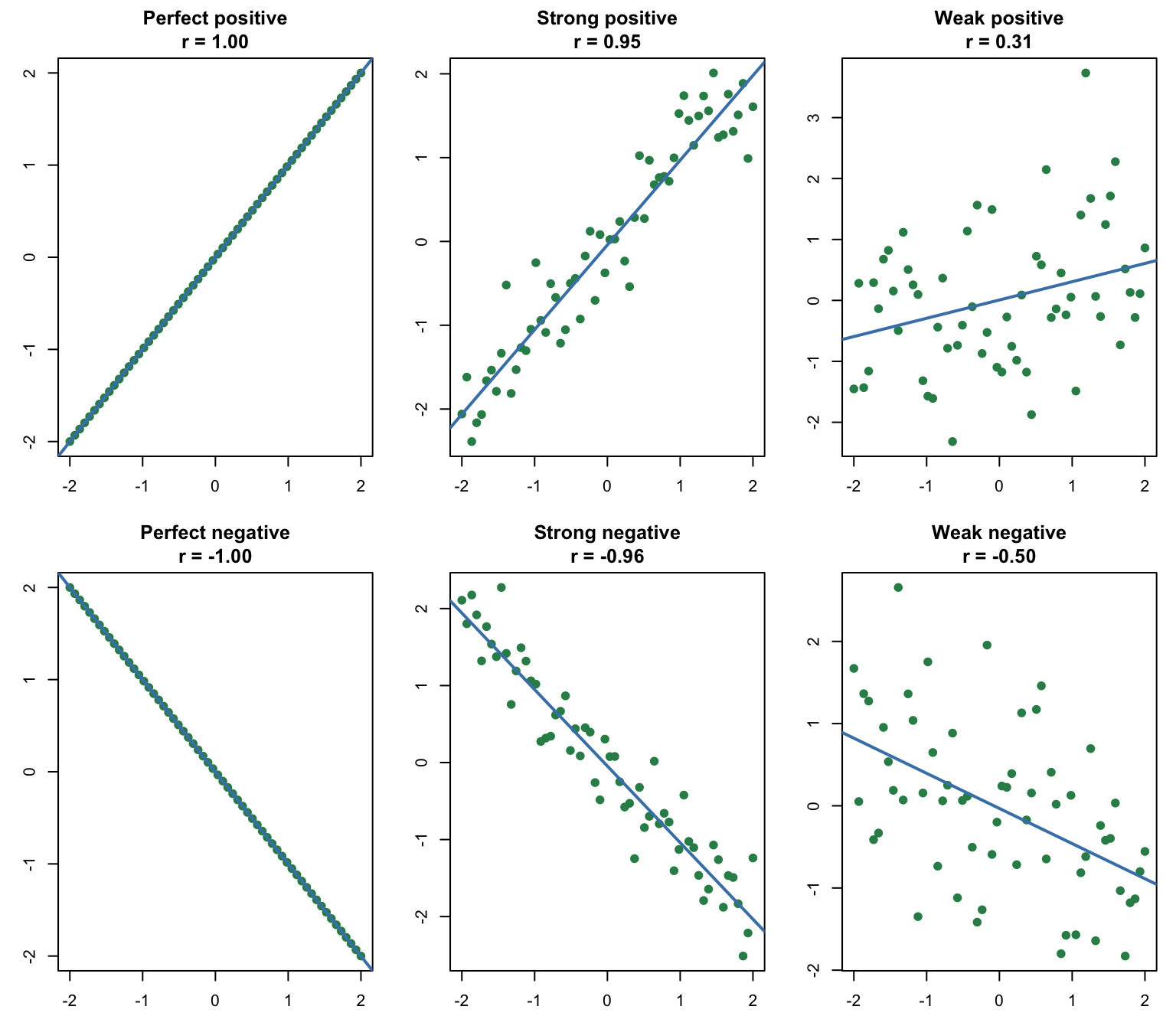
The sign describes direction and the magnitude describes the strength of a linear relationship:

Correlation Interpretation
\(\rho=1\) Perfect positive linear relationship
\(0<\rho<1\) Positive linear association
\(\rho=0\) No linear association; a nonlinear relationship may remain
\(-1<\rho<0\) Negative linear association
\(\rho=-1\) Perfect negative linear relationship

Correlation has no units and is unchanged by positive changes of scale and location. Multiplying exactly one variable by a negative number reverses its sign.

Code
weighted_correlation <- function(x, y, probability) {
  mean_x <- sum(x * probability)
  mean_y <- sum(y * probability)
  covariance <- sum(
    (x - mean_x) * (y - mean_y) * probability
  )
  variance_x <- sum((x - mean_x)^2 * probability)
  variance_y <- sum((y - mean_y)^2 * probability)
  covariance / sqrt(variance_x * variance_y)
}

rho_original <- with(
  joint_grid,
  weighted_correlation(X, Y, probability)
)
rho_positive_rescaling <- with(
  joint_grid,
  weighted_correlation(100 * X + 5, 2 * Y - 10, probability)
)
rho_sign_reversal <- with(
  joint_grid,
  weighted_correlation(-X, Y, probability)
)

c(
  original = rho_original,
  positive_rescaling = rho_positive_rescaling,
  sign_reversal = rho_sign_reversal
)
          original positive_rescaling      sign_reversal 
         0.2182179          0.2182179         -0.2182179 

Correlation patterns in fictional data

The following simulation extends the deck’s correlation sketches. The same \(X\) values are paired with different amounts of noise to show why points spread farther from a straight line as \(|r|\) decreases.

Code
set.seed(14270)
n <- 60
x_sim <- seq(-2, 2, length.out = n)

patterns <- list(
  "Perfect positive" = x_sim,
  "Strong positive" = x_sim + rnorm(n, sd = 0.35),
  "Weak positive" = 0.35 * x_sim + rnorm(n, sd = 1),
  "Perfect negative" = -x_sim,
  "Strong negative" = -x_sim + rnorm(n, sd = 0.35),
  "Weak negative" = -0.35 * x_sim + rnorm(n, sd = 1)
)

old_par <- par(mfrow = c(2, 3), mar = c(3, 3, 3, 1))
for (label in names(patterns)) {
  y_sim <- patterns[[label]]
  plot(
    x_sim,
    y_sim,
    pch = 19,
    col = "seagreen4",
    xlab = "X",
    ylab = "Y",
    main = sprintf("%s\nr = %.2f", label, cor(x_sim, y_sim))
  )
  abline(lm(y_sim ~ x_sim), col = "steelblue", lwd = 2)
}

Code
par(old_par)

Practice questions

  1. From the joint table, compute \(P(X=3)\), \(P(Y=4)\), and \(P(X=3,Y=4)\).
  2. Compute \(P(X=3\mid Y=4)\). Does it equal \(P(X=3)\)?
  3. Verify \(\operatorname{Var}(Y)=0.84\) from the marginal PMF of \(Y\).
  4. If \(U=5X+2\) and \(V=-3Y+1\), find \(\operatorname{Cov}(U,V)\) and \(\operatorname{Corr}(U,V)\).
  5. Give a short reason why \(\rho=0\) does not prove independence.
  1. The probabilities are \(0.5\), \(0.7\), and \(0.4\), respectively.
  2. \(P(X=3\mid Y=4)=0.4/0.7\approx0.571\), which is not \(P(X=3)=0.5\).
  3. \(E(Y^2)=2^2(0.3)+4^2(0.7)=12.4\), so \(\operatorname{Var}(Y)=12.4-3.4^2=0.84\).
  4. \(\operatorname{Cov}(U,V)=5(-3)(0.2)=-3\). Because exactly one scale factor is negative, \(\operatorname{Corr}(U,V)=-0.2182\) approximately.
  5. Correlation detects linear association only. For example, \(Y=X^2\) with a symmetric \(X\) can have covariance and correlation 0 while \(Y\) is fully determined by \(X\).