Course: Statistics and Probability for Data Science (DS14270).
Source deck: Samer El Kababji, SD07 — Sampling Distributions and Inference.
Maximum likelihood estimation (MLE) treats the observed data as fixed and asks which parameter value makes those data most likely.
Likelihood and log-likelihood
For an i.i.d. sample \(x_1,\ldots,x_n\) from a PMF or PDF \(f(x;\theta)\), the likelihood is
\[
L(\theta)=\prod_{i=1}^n f(x_i;\theta).
\]
An MLE \(\widehat\theta\) maximizes \(L(\theta)\). Because logarithms are strictly increasing, it equivalently maximizes
\[
\ell(\theta)=\log L(\theta)
=\sum_{i=1}^n\log f(x_i;\theta).
\]
The sum is easier to calculate and is numerically more stable than a product of many small probabilities.
Poisson MLE
For \(X_i\sim\operatorname{Poisson}(\lambda)\),
\[
P(X_i=x_i;\lambda)=e^{-\lambda}\frac{\lambda^{x_i}}{x_i!}.
\]
Independence gives
\[
L(\lambda)
=\prod_{i=1}^n e^{-\lambda}\frac{\lambda^{x_i}}{x_i!}
=\frac{e^{-n\lambda}\lambda^{\sum_i x_i}}
{\prod_i x_i!}.
\]
The log-likelihood is
\[
\ell(\lambda)
=-n\lambda+\left(\sum_i x_i\right)\log\lambda
-\sum_i\log(x_i!).
\]
Differentiating and setting the result to zero,
\[
\ell'(\lambda)=-n+\frac{\sum_i x_i}{\lambda}=0
\quad\Longrightarrow\quad
\widehat\lambda=\frac1n\sum_i x_i=\bar x.
\]
Code
poisson_data <- c(2, 4, 3, 1, 5, 2, 3, 4)
lambda_hat <- mean(poisson_data)

poisson_loglik <- function(lambda, x) {
  sum(dpois(x, lambda = lambda, log = TRUE))
}

c(
  analytic_MLE = lambda_hat,
  numerical_MLE = optimize(
    poisson_loglik,
    interval = c(0.001, 10),
    x = poisson_data,
    maximum = TRUE
  )$maximum
)
 analytic_MLE numerical_MLE
     3.000000      3.000015
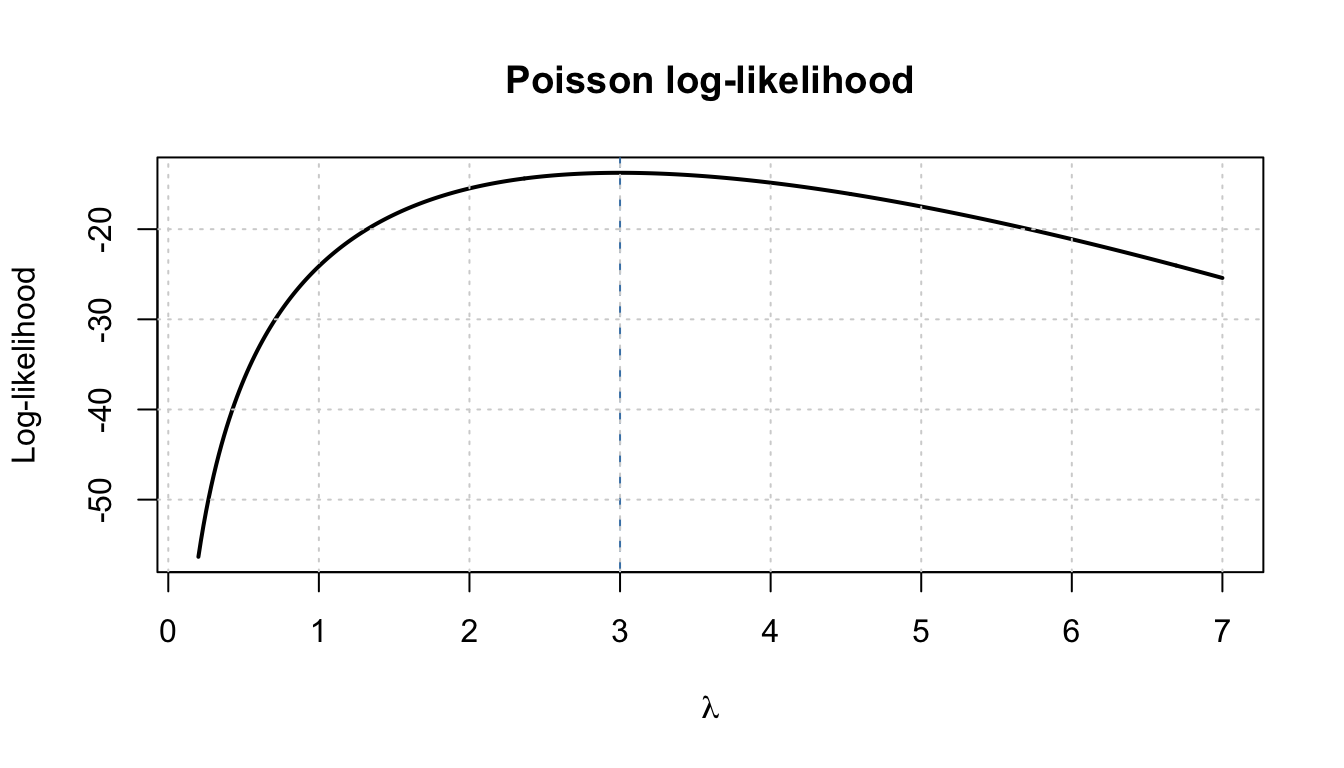
Code
lambda_grid <- seq(0.2, 7, length.out = 400)
loglik_values <- vapply(
  lambda_grid, poisson_loglik, numeric(1), x = poisson_data
)

plot(
  lambda_grid, loglik_values, type = "l", lwd = 2,
  xlab = expression(lambda), ylab = "Log-likelihood",
  main = "Poisson log-likelihood"
)
abline(v = lambda_hat, col = "steelblue", lty = 2)
grid()
Exponential rate MLE
For \(X_i\sim\operatorname{Exp}(\lambda)\) with rate \(\lambda\),
\[
f(x_i;\lambda)=\lambda e^{-\lambda x_i},\qquad x_i\geq0.
\]
Thus
\[
L(\lambda)=\lambda^n e^{-\lambda\sum_i x_i},
\]
and
\[
\ell(\lambda)=n\log\lambda-\lambda\sum_i x_i.
\]
Solving the score equation,
\[
\ell'(\lambda)=\frac n\lambda-\sum_i x_i=0
\quad\Longrightarrow\quad
\widehat\lambda=\frac n{\sum_i x_i}=\frac1{\bar x}.
\]
Code
waiting_times <- c(0.8, 1.4, 0.6, 2.2, 1.0, 0.9)
rate_hat <- 1 / mean(waiting_times)

exponential_loglik <- function(rate, x) {
  sum(dexp(x, rate = rate, log = TRUE))
}

c(
  analytic_MLE = rate_hat,
  numerical_MLE = optimize(
    exponential_loglik,
    interval = c(0.001, 10),
    x = waiting_times,
    maximum = TRUE
  )$maximum
)
 analytic_MLE numerical_MLE
    0.8695652     0.8695727
The estimated exponential mean is \(1/\widehat\lambda=\bar x\). Keep rate and scale conventions explicit.
Why verify the maximum?
For both examples, the second derivative is negative at every positive parameter value:
\[
\ell''_{\text{Poisson}}(\lambda)
=-\frac{\sum_i x_i}{\lambda^2}<0,
\]
\[
\ell''_{\text{Exponential}}(\lambda)
=-\frac n{\lambda^2}<0.
\]
Therefore the stationary point is a maximum, provided the sample is not a boundary case such as all-zero Poisson counts.
Simulation behavior (fictional extension)
Code
set.seed(14270)
true_lambda <- 3
n <- 50
repetitions <- 10000

poisson_estimates <- replicate(
  repetitions,
  mean(rpois(n, lambda = true_lambda))
)

c(
  true_lambda = true_lambda,
  average_MLE = mean(poisson_estimates),
  empirical_sd = sd(poisson_estimates),
  theoretical_sd = sqrt(true_lambda / n)
)
   true_lambda    average_MLE   empirical_sd theoretical_sd
     3.0000000      2.9970200      0.2423606      0.2449490
Practice questions
- For Poisson counts \(1,0,2,3,4\), find \(\widehat\lambda\).
- Write the Poisson log-likelihood up to terms that do not depend on \(\lambda\).
- For exponential waiting times \(2,1,3,4\), find the MLE of the rate.
- Why is the log-likelihood usually preferred computationally?
- The MLE is the sample mean: \((1+0+2+3+4)/5=2\).
- \(\ell(\lambda)=-5\lambda+10\log\lambda+C\).
- \(\widehat\lambda=4/(2+1+3+4)=0.4\).
- Products become sums, derivatives are simpler, and sums of log probabilities avoid numerical underflow.