Code
call_outcomes <- c("Success", "Failure")
X_call <- c(Success = 1, Failure = 0)

data.frame(
  outcome = call_outcomes,
  X = unname(X_call[call_outcomes])
)
outcome X
1 Success 1
2 Failure 0
SD04 — Random Variables
Course: Statistics and Probability for Data Science (DS14270).
Source deck: Samer El Kababji, SD04 — Random Variables.
This lesson develops the deck’s distinction between discrete and continuous random variables and connects probability mass, probability density, and cumulative distribution functions. The practice questions and computational checks extend the deck’s examples.
A random variable is a function from a sample space \(S\) to the real numbers:
\[ X:S\longrightarrow\mathbb{R}. \]
The randomness is in the outcome \(\omega\in S\); once \(\omega\) is known, the value \(X(\omega)\) is determined. For a phone call with outcomes Success and Failure, one possible random variable is
\[ X(\text{Success})=1, \qquad X(\text{Failure})=0. \]
call_outcomes <- c("Success", "Failure")
X_call <- c(Success = 1, Failure = 0)
data.frame(
outcome = call_outcomes,
X = unname(X_call[call_outcomes])
) outcome X
1 Success 1
2 Failure 0Now test 9-volt batteries until the first acceptable battery, denoted \(S\), appears. With \(F\) denoting failure,
\[ S=\{S,FS,FFS,FFFS,\ldots\}, \]
and the number tested is
\[ X(S)=1,\quad X(FS)=2,\quad X(FFS)=3,\quad\ldots. \]
battery_outcomes <- c("S", "FS", "FFS", "FFFS")
number_tested <- nchar(battery_outcomes)

data.frame(
  outcome = battery_outcomes,
  X = number_tested
)
outcome X
1 S 1
2 FS 2
3 FFS 3
4 FFFS 4A discrete random variable has a finite or countably infinite set of possible values. Counts such as customers per hour, students passing an exam, or emails per day are discrete.
A continuous random variable can take values throughout an interval. Completion time, temperature, weight, and rainfall amount are continuous.
For a continuous variable, a single point has zero probability even though an interval can have positive probability:
\[ P(X=x)=0, \qquad P(a\leq X\leq b)>0\ \text{may hold}. \]
The following draws illustrate the different supports. The simulations are fictional extensions of the deck.
set.seed(14270)

customers_per_hour <- rpois(8, lambda = 12)
completion_time <- rexp(8, rate = 0.5)

data.frame(
  discrete_count = customers_per_hour,
  continuous_time = round(completion_time, 3)
)
discrete_count continuous_time
1 11 0.348
2 15 3.645
3 18 0.200
4 16 4.257
5 13 6.855
6 24 1.109
7 10 4.920
8 12 0.707For a discrete random variable \(X\), its probability mass function (PMF) is
\[ p(x)=P(X=x) =P\bigl(\{\omega\in S:X(\omega)=x\}\bigr). \]
A valid PMF satisfies
\[ p(x)\geq0 \quad\text{and}\quad \sum_x p(x)=1. \]
Six equally likely boxes contain respectively \(0,2,0,1,2,0\) defective components. If \(X\) is the number of defectives in the selected box, then
\[ p(0)=\frac36=0.5, \qquad p(1)=\frac16, \qquad p(2)=\frac26=\frac13. \]
defects <- c(0, 2, 0, 1, 2, 0)
pmf_boxes <- prop.table(table(defects))

pmf_boxes
defects
0 1 2
0.5000000 0.1666667 0.3333333 sum(pmf_boxes)[1] 1stopifnot(isTRUE(all.equal(sum(pmf_boxes), 1)))The PMF groups sample points that produce the same value of \(X\). Here three different boxes all map to \(X=0\).
For a continuous random variable \(X\), a probability density function (PDF) \(f\) satisfies
\[ f(x)\geq0, \qquad \int_{-\infty}^{\infty}f(x)\,dx=1. \]
Probabilities are areas under the density:
\[ P(a\leq X\leq b)=\int_a^b f(x)\,dx. \]
Unlike a PMF value, \(f(x)\) is not the probability of the point \(x\). A density may even exceed 1 as long as its total area is 1.
The deck gives the density
\[ f(x)= \begin{cases} \dfrac{2}{(x+1)^3}, & x\geq0,\\[4pt] 0, & x<0. \end{cases} \]
It is normalized because
\[ \int_0^\infty\frac{2}{(x+1)^3}\,dx =\left[-\frac{1}{(x+1)^2}\right]_0^\infty=1. \]
For example,
\[ P(1\leq X\leq3) =\int_1^3\frac{2}{(x+1)^3}\,dx =\frac{3}{16}=0.1875. \]
battery_pdf <- function(x) {
  ifelse(x >= 0, 2 / (x + 1)^3, 0)
}

total_area <- integrate(battery_pdf, lower = 0, upper = Inf)$value
P_between_1_and_3 <- integrate(battery_pdf, lower = 1, upper = 3)$value

c(total_area = total_area,
  P_between_1_and_3 = P_between_1_and_3)
total_area P_between_1_and_3
1.0000 0.1875 stopifnot(isTRUE(all.equal(P_between_1_and_3, 3 / 16)))curve(
battery_pdf,
from = 0,
to = 7,
n = 501,
lwd = 2,
col = "steelblue",
xlab = "x (hours)",
ylab = "f(x)",
main = "Battery time-to-failure density"
)
grid()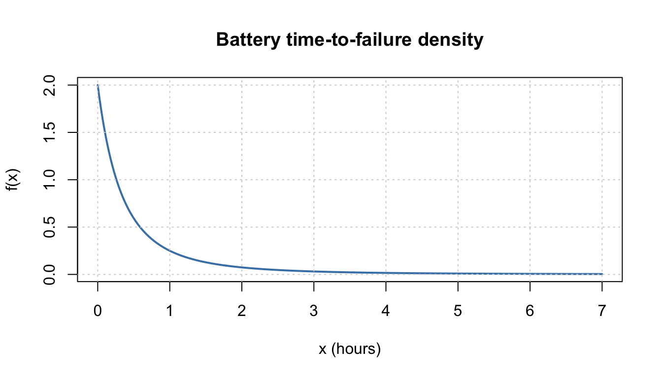
The cumulative distribution function (CDF) works for every random variable:
\[ F(x)=P(X\leq x). \]
The standard definition includes equality. For a continuous random variable, \(P(X=x)=0\), so \(P(X\leq x)=P(X<x)\). Every CDF is nondecreasing, right-continuous, and satisfies
\[ \lim_{x\to-\infty}F(x)=0, \qquad \lim_{x\to\infty}F(x)=1. \]
For a discrete random variable,
\[ F(x)=\sum_{y\leq x}p(y), \qquad p(x)=F(x)-F(x^-), \]
where \(F(x^-)\) is the value immediately to the left of \(x\). For a continuous random variable,
\[ F(x)=\int_{-\infty}^x f(u)\,du, \qquad f(x)=F'(x) \]
where the derivative exists.
Let \(Y\) be purchased memory capacity in GB, with PMF
| \(y\) | 1 | 2 | 4 | 8 | 16 |
|---|---|---|---|---|---|
| \(p(y)\) | 0.05 | 0.10 | 0.35 | 0.40 | 0.10 |
The cumulative probabilities are
\[ F(1)=0.05,\quad F(2)=0.15,\quad F(4)=0.50, \quad F(8)=0.90,\quad F(16)=1. \]
Between possible values, the CDF is constant. Thus
\[ F(2.7)=F(2)=0.15, \qquad F(7.999)=F(4)=0.50. \]
capacity <- c(1, 2, 4, 8, 16)
capacity_pmf <- c(0.05, 0.10, 0.35, 0.40, 0.10)
capacity_cdf <- cumsum(capacity_pmf)

F_capacity <- function(q) {
  vapply(q, function(value) {
    sum(capacity_pmf[capacity <= value])
  }, numeric(1))
}

data.frame(capacity, capacity_pmf, capacity_cdf)
capacity capacity_pmf capacity_cdf
1 1 0.05 0.05
2 2 0.10 0.15
3 4 0.35 0.50
4 8 0.40 0.90
5 16 0.10 1.00F_capacity(c(2.7, 7.999, 16))[1] 0.15 0.50 1.00plot(
stepfun(capacity, c(0, capacity_cdf)),
verticals = FALSE,
do.points = TRUE,
pch = 19,
xlab = "Memory capacity y (GB)",
ylab = "F(y)",
main = "CDF of purchased flash-drive capacity"
)
grid()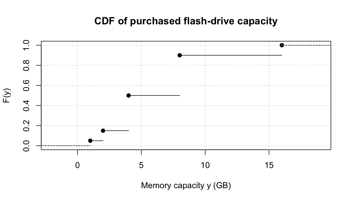
Suppose independent trials have success probability \(p\), and \(X\) is the trial number of the first success. Then
\[ P(X=x)=(1-p)^{x-1}p, \qquad x=1,2,3,\ldots. \]
Summing the geometric series gives
\[ F(x)=P(X\leq x) =1-(1-p)^{\lfloor x\rfloor}, \qquad x\geq1, \]
and \(F(x)=0\) for \(x<1\).
R’s geometric distribution counts failures before the first success, so the deck’s \(X\) equals the R value plus 1.
p_success <- 0.51
x <- 1:6

geometric_table <- data.frame(
  x = x,
  pmf_formula = (1 - p_success)^(x - 1) * p_success,
  pmf_R = dgeom(x - 1, prob = p_success),
  cdf_formula = 1 - (1 - p_success)^x,
  cdf_R = pgeom(x - 1, prob = p_success)
)

geometric_table
x pmf_formula pmf_R cdf_formula cdf_R
1 1 0.51000000 0.51000000 0.5100000 0.5100000
2 2 0.24990000 0.24990000 0.7599000 0.7599000
3 3 0.12245100 0.12245100 0.8823510 0.8823510
4 4 0.06000099 0.06000099 0.9423520 0.9423520
5 5 0.02940049 0.02940049 0.9717525 0.9717525
6 6 0.01440624 0.01440624 0.9861587 0.9861587stopifnot(with(geometric_table,
isTRUE(all.equal(pmf_formula, pmf_R)) &&
isTRUE(all.equal(cdf_formula, cdf_R))))Let \(X\) be weekly gravel sales in tons with density
\[ f(x)= \begin{cases} \dfrac32(1-x^2), & 0\leq x\leq1,\\[4pt] 0, & \text{otherwise}. \end{cases} \]
For \(0\leq x\leq1\),
\[ F(x)=\int_0^x\frac32(1-u^2)\,du =\frac32\left(x-\frac{x^3}{3}\right). \]
Therefore the complete CDF is
\[ F(x)= \begin{cases} 0, & x<0,\\[2pt] \dfrac32\left(x-\dfrac{x^3}{3}\right), & 0\leq x\leq1,\\[6pt] 1, & x>1. \end{cases} \]
gravel_pdf <- function(x) {
  ifelse(x >= 0 & x <= 1, 3 / 2 * (1 - x^2), 0)
}

gravel_cdf <- function(x) {
  ifelse(
    x < 0,
    0,
    ifelse(x <= 1, 3 / 2 * (x - x^3 / 3), 1)
  )
}

check_points <- c(0, 0.25, 0.5, 0.75, 1)
cbind(
  x = check_points,
  formula = gravel_cdf(check_points),
  integration = vapply(
    check_points,
    function(q) integrate(gravel_pdf, -Inf, q)$value,
    numeric(1)
  )
)
x formula integration
[1,] 0.00 0.0000000 0.0000000
[2,] 0.25 0.3671875 0.3671875
[3,] 0.50 0.6875000 0.6875000
[4,] 0.75 0.9140625 0.9140647
[5,] 1.00 1.0000000 1.0000000