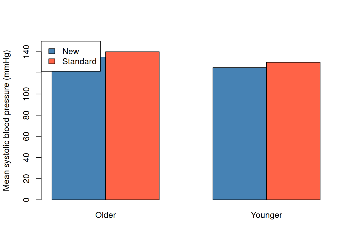
medication age_group patients mean_bp
1   Standard   Younger       20     130
2   Standard     Older       80     140
3        New   Younger       90     125
4        New     Older       10     135
Age group is a covariate because it is an additional variable that may help us understand differences in blood pressure.
Comparing the two medication groups
The overall mean blood pressure for each medication combines its younger and older patients. Each age group contributes according to its patient count:
Here \(j\) runs over the age groups within one medication, \(n_j\) is the patient count, and \(\bar y_j\) is that age group’s mean blood pressure. Apply the equation separately for New and Standard.
Worked example — comparing medications. For New, combine 90 younger patients with a mean of 125 mmHg and 10 older patients with a mean of 135 mmHg:
These calculations produce the table below: weighted_bp is the numerator, patients is the denominator, and mean_bp is their quotient. Younger and older patients are combined within each medication, giving one row for New and one for Standard.
The new-medication group has an average blood pressure 12 mmHg lower than the standard-medication group. This is an association in the observed data. It does not yet tell us how much of the difference was caused by the medication.
How age can confuse the comparison
The treatment groups have very different age compositions.
Code
age_counts <-xtabs(patients ~ medication + age_group, data = blood_pressure)age_counts
          age_group
medication Older Younger
  New         10      90
  Standard    80      20
Code
prop.table(age_counts, margin =1)
          age_group
medication Older Younger
  New        0.1     0.9
  Standard   0.8     0.2
Most patients receiving the standard medication are older, while most patients receiving the new medication are younger. Older patients also have higher blood pressure in both medication groups. Age is therefore connected to both:
which medication patients received; and
their blood pressure.
In this example, age is a confounder. It mixes the medication comparison with an age comparison.
Compare similar patients
We can compare medications separately within each age group:
\[
\text{difference within an age group}
=\bar y_{\text{New}}-\bar y_{\text{Standard}}.
\]
Worked example — compare within each age group. For younger patients, \(125-130=-5\) mmHg; for older patients, \(135-140=-5\) mmHg. A negative difference means the new-medication group has lower average blood pressure.
This simple separation by age is useful for explaining confounding. In a real study, many covariates may matter at the same time, and some age groups may contain very few patients. More advanced statistical methods are then needed.
Association and causation
Two variables are associated when their values tend to differ together. An association can be measured from observational data, but it does not by itself show that changing one variable will change the other.
A causal effect asks a different question: what would happen to the same kind of patients under the new medication compared with the standard medication? We cannot give both medications to the same person under identical conditions, so study design matters.
In a randomized experiment, chance assigns the treatment. This helps make the treatment groups similar in age and other characteristics before treatment. An observational study can reveal useful associations, but differences between the groups may provide other explanations for the result.
The lesson from this example is:
compare similar groups when possible;
look for variables connected to both the treatment and response; and
do not describe an observed association as a causal effect without support from the study design and assumptions.
Try it: change the number of older and younger patients so both medication groups have the same age composition. Recalculate the overall difference.