Code
set.seed(14270)
sample_size <- 10
one_sample <- rweibull(sample_size, shape = 2, scale = 5)

c(sample_mean = mean(one_sample), sample_sd = sd(one_sample))
sample_mean sample_sd
4.819165 2.635624 
SD07 — Sampling Distributions and Inference
Course: Statistics and Probability for Data Science (DS14270).
Source deck: Samer El Kababji, SD07 — Sampling Distributions and Inference.
This lesson distinguishes observations from sample means, derives the sample mean’s center and spread, and uses the central limit theorem (CLT).
For an i.i.d. sample \(X_1,\ldots,X_n\) from a population with mean \(\mu\) and variance \(\sigma^2\),
\[ \overline X=\frac1n\sum_{i=1}^nX_i. \]
Different random samples produce different values of \(\overline X\). Its distribution across all possible samples is the sampling distribution.
set.seed(14270)
sample_size <- 10
one_sample <- rweibull(sample_size, shape = 2, scale = 5)
c(sample_mean = mean(one_sample), sample_sd = sd(one_sample))sample_mean sample_sd
4.819165 2.635624 The deck introduces a Weibull population with shape 2 and scale 5. Its population moments are
\[ \mu=5\Gamma(1+1/2)\approx4.4311, \]
\[ \sigma^2=5^2\left[\Gamma(2)-\Gamma(1.5)^2\right]\approx5.365. \]
shape <- 2
scale <- 5
mu <- scale * gamma(1 + 1 / shape)
variance <- scale^2 * (
  gamma(1 + 2 / shape) - gamma(1 + 1 / shape)^2
)

c(mean = mu, variance = variance, sd = sqrt(variance))
mean variance sd
4.431135 5.365046 2.316257 Linearity of expectation gives
\[ E(\overline X) =\frac1n\sum_{i=1}^nE(X_i)=\mu. \]
Independence makes the variances add:
\[ \operatorname{Var}(\overline X) =\frac1{n^2}\sum_{i=1}^n\operatorname{Var}(X_i) =\frac{\sigma^2}{n}. \]
The standard deviation of the sampling distribution is the standard error:
\[ \operatorname{SE}(\overline X)=\frac{\sigma}{\sqrt n}. \]
n <- c(1, 5, 10, 30, 100)
data.frame(
  sample_size = n,
  expected_sample_mean = mu,
  standard_error = sqrt(variance) / sqrt(n)
)
sample_size expected_sample_mean standard_error
1 1 4.431135 2.3162569
2 5 4.431135 1.0358616
3 10 4.431135 0.7324647
4 30 4.431135 0.4228887
5 100 4.431135 0.2316257If every \(X_i\sim N(\mu,\sigma^2)\) independently, then for every sample size
\[ \overline X\sim N\left(\mu,\frac{\sigma^2}{n}\right). \]
mu_normal <- 20
sigma_normal <- 6
n <- 9

c(
  sample_mean_mean = mu_normal,
  sample_mean_variance = sigma_normal^2 / n,
  sample_mean_sd = sigma_normal / sqrt(n)
)
sample_mean_mean sample_mean_variance sample_mean_sd
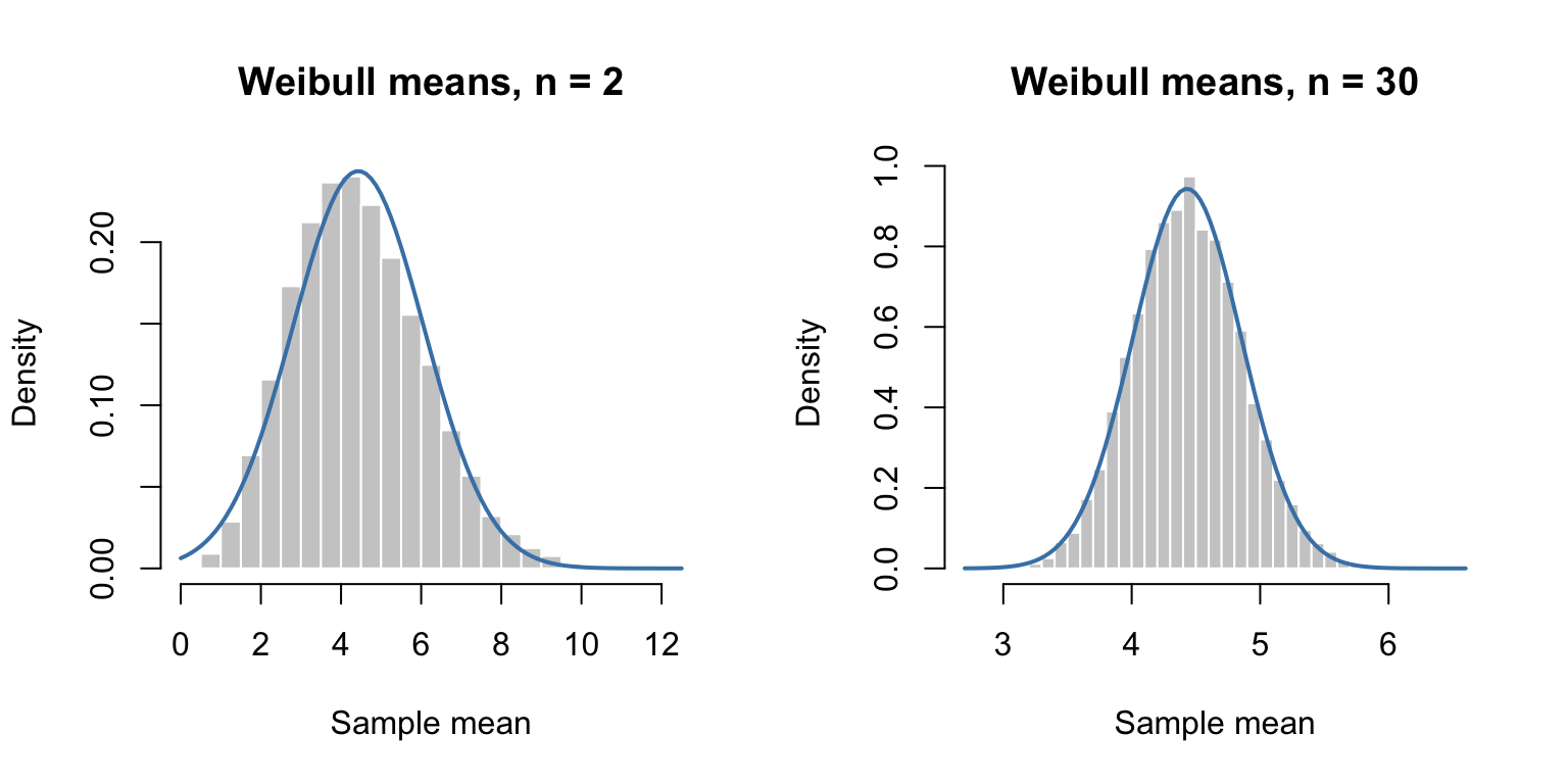
20 4 2 For i.i.d. observations with finite mean and variance, as \(n\) increases,
\[ \frac{\overline X-\mu}{\sigma/\sqrt n} \overset{d}{\longrightarrow}N(0,1). \]
Equivalently, for sufficiently large \(n\),
\[ \overline X\ \dot\sim\ N\left(\mu,\frac{\sigma^2}{n}\right), \]
even when the population is not normal. The deck uses \(n\geq30\) as a common rule of thumb, not a guarantee for every population.
set.seed(14270)
repetitions <- 20000
sample_sizes <- c(2, 30)

old_par <- par(mfrow = c(1, 2))
for (n in sample_sizes) {
  sample_means <- replicate(
    repetitions,
    mean(rweibull(n, shape = 2, scale = 5))
  )
  hist(
    sample_means, probability = TRUE, breaks = 40,
    col = "grey80", border = "white",
    main = paste("Weibull means, n =", n), xlab = "Sample mean"
  )
  curve(
    dnorm(x, mean = mu, sd = sqrt(variance / n)),
    add = TRUE, col = "steelblue", lwd = 2
  )
}
par(old_par)The population has mean 4.0 g and standard deviation 1.5 g. For \(n=50\),
\[ \operatorname{SE}(\overline X)=\frac{1.5}{\sqrt{50}}\approx0.2121. \]
The CLT gives
\[ P(3.5\leq\overline X\leq3.8) \approx \Phi\left(\frac{3.8-4}{1.5/\sqrt{50}}\right) -\Phi\left(\frac{3.5-4}{1.5/\sqrt{50}}\right). \]
mu <- 4
sigma <- 1.5
n <- 50
se <- sigma / sqrt(n)
z_lower <- (3.5 - mu) / se
z_upper <- (3.8 - mu) / se

c(
  standard_error = se,
  z_lower = z_lower,
  z_upper = z_upper,
  probability = pnorm(z_upper) - pnorm(z_lower),
  rounded_table_probability = pnorm(-0.94) - pnorm(-2.36)
)
standard_error z_lower z_upper
0.2121320 -2.3570226 -0.9428090
probability rounded_table_probability
0.1636782 0.1644713 R’s unrounded calculation is about \(0.1649\); the deck’s rounded z-table calculation is \(0.1645\).
pnorm(83, 80, 2) - pnorm(78, 80, 2) gives approximately \(0.7745\).