Course: Statistics and Probability for Data Science (DS14270). Source deck: Samer El Kababji, SD02 — Exploratory Data Analysis.
Different plots answer different questions. This lesson uses base R and the built-in iris dataset, together with one small fictional categorical dataset.
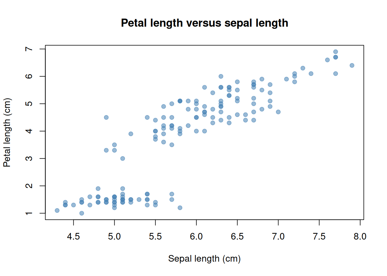
Two numerical variables: scatter plot
For observation \(i\), a scatter plot places one point at the coordinate
\[
(x_i,y_i).
\]
Worked example — one flower, one point. The first iris record has sepal length 5.1 cm and petal length 1.4 cm. Its point is \((x_1,y_1)=(5.1,1.4)\): move to 5.1 horizontally and 1.4 vertically.
The horizontal position represents one numerical variable and the vertical position represents another. Here each point is one iris flower.
Read a scatter plot by looking for direction, form, strength, clusters, gaps, and unusual observations. The visible association does not by itself establish that changing sepal length would cause petal length to change.
Add a descriptive smooth
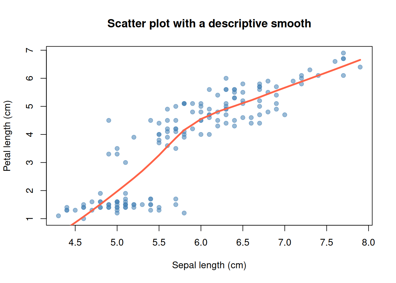
A smooth curve can help reveal the overall shape when many points overlap. lowess() estimates local typical values using nearby observations. It is a descriptive guide rather than a causal conclusion.
Code
plot(iris$Sepal.Length, iris$Petal.Length,pch =19, col =rgb(70, 130, 180, 140, maxColorValue =255),xlab ="Sepal length (cm)", ylab ="Petal length (cm)",main ="Scatter plot with a descriptive smooth")smooth_curve <-lowess(iris$Sepal.Length, iris$Petal.Length)lines(smooth_curve, col ="tomato", lwd =3)
The smooth summarizes the observed pattern. It should not hide clusters or replace inspection of the original points.
One categorical variable: counts and proportions
For category \(c\), the frequency and sample proportion are
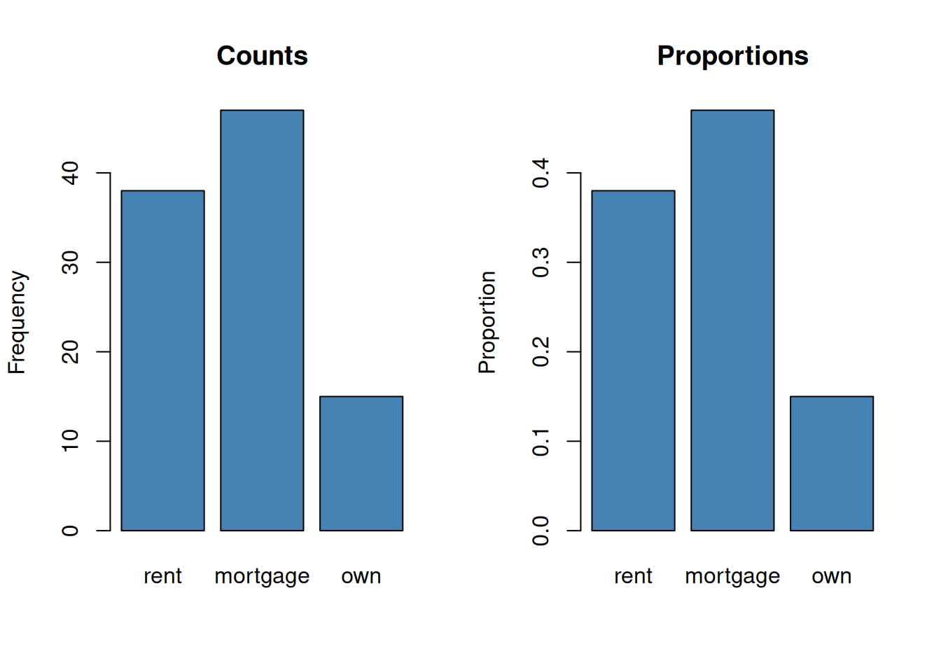
Worked example — category indicators and proportions. In the tiny sequence (rent, own, rent, mortgage, rent), the indicators for rent are \((1,0,1,0,1)\), so \(n_{\text{rent}}=1+0+1+0+1=3\) and \(\widehat p_{\text{rent}}=3/5=0.60\). In the larger dataset below, the same rule gives \(38/100=0.38\) for rent, \(47/100=0.47\) for mortgage, and \(15/100=0.15\) for own; the proportions sum to 1.
A bar plot can display either counts or proportions. Bar plots leave space between categories because the horizontal positions are labels, not a continuous number line.
Code
old_mfrow <-par("mfrow")par(mfrow =c(1, 2))barplot(category_counts, col ="steelblue", ylab ="Frequency",main ="Counts")barplot(category_proportions, col ="steelblue", ylab ="Proportion",main ="Proportions")
Code
par(mfrow = old_mfrow)
The plots have the same shape because every count was divided by the same total. The vertical scales answer different questions.
Numerical response across categories: box plots
To compare a numerical variable across groups, compute a separate five-number summary for each category:
Worked example — summarize one group. Suppose one category has ordered values \((3,5,8,9,14,21)\). With type = 7 quartiles, its five-number summary is
\[
(3,\ 5.75,\ 8.5,\ 12.75,\ 21).
\]
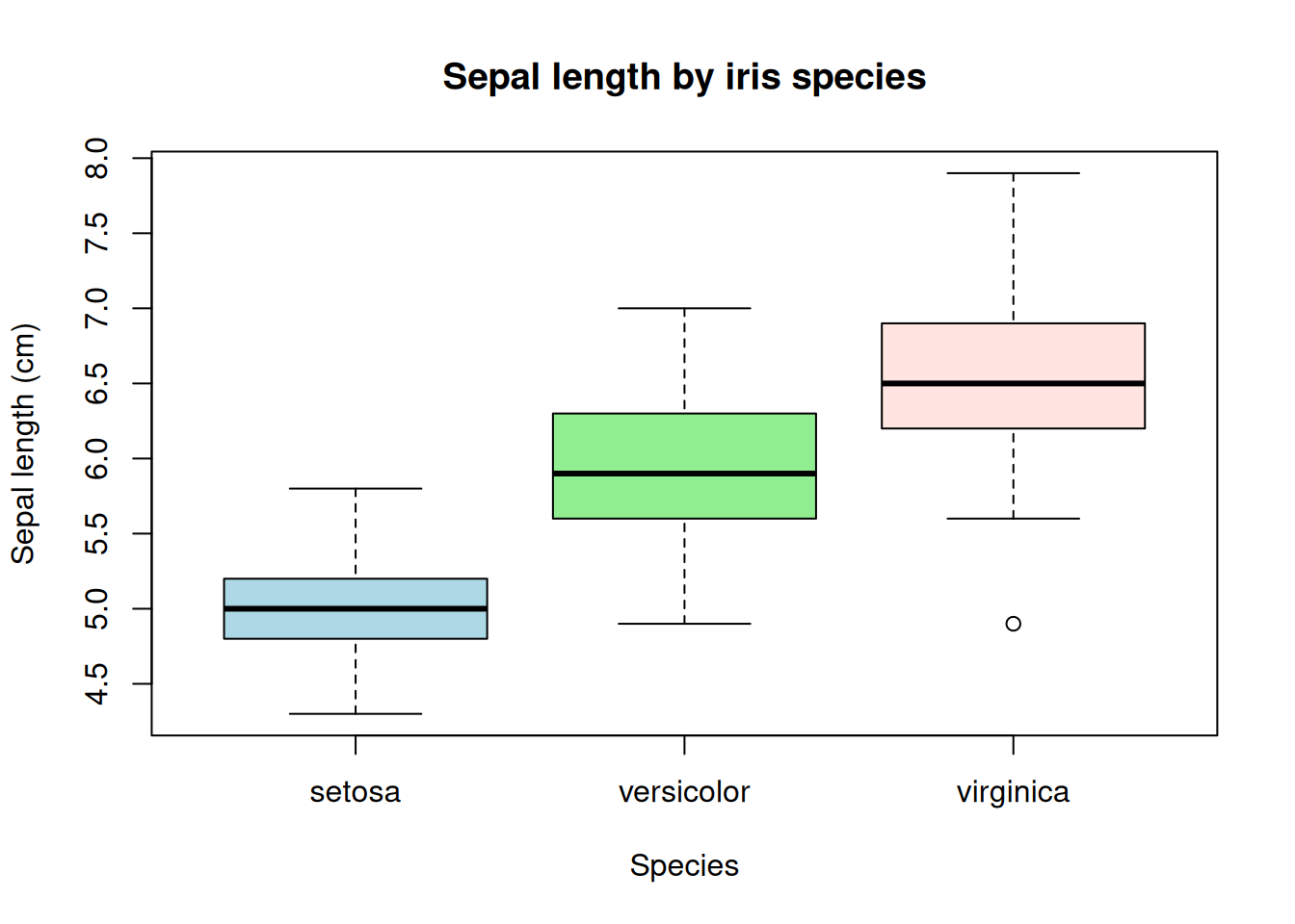
The minimum and maximum are the endpoints, the median is \((8+9)/2=8.5\), and the quartiles interpolate at positions 2.25 and 4.75. Repeat the calculation separately for each category. Box-plot whiskers reach the most extreme observations within their outlier fences; they need not equal the minimum and maximum when outliers are present.
Code
sepal_by_species <-split(iris$Sepal.Length, iris$Species)group_summaries <-do.call(rbind, lapply(sepal_by_species, function(values) {c(minimum =min(values),Q1 =unname(quantile(values, 0.25, type =7)),median =median(values),Q3 =unname(quantile(values, 0.75, type =7)),maximum =max(values))}))group_summaries
boxplot(Sepal.Length ~ Species, data = iris,col =c("lightblue", "lightgreen", "mistyrose"),xlab ="Species", ylab ="Sepal length (cm)",main ="Sepal length by iris species")
Box plots make medians, quartiles, and suspected outliers easy to compare, but they hide many details of the shape inside each group.
Box plots and violin plots
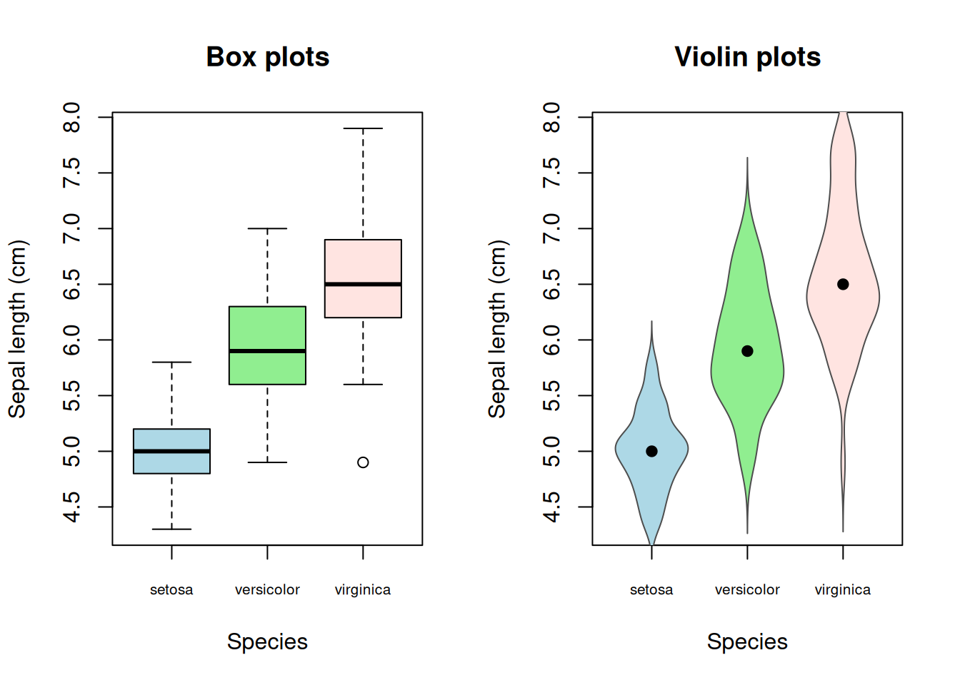
A violin plot uses a smooth density estimate \(\widehat f_g(y)\) for each group \(g\). At height \(y\), the violin width is proportional to \(\widehat f_g(y)\). Wider sections indicate values that occur more densely.
Worked example — convert density to width. The helper below scales each violin’s largest density to a half-width of 0.38:
If the maximum estimated density in one group is 0.8 and the density at a particular height is 0.4, its half-width there is \(0.38(0.4/0.8)=0.19\). Around a category centered at 2, the left and right edges are \(2-0.19=1.81\) and \(2+0.19=2.19\). These density values are illustrative; each group’s actual estimates come from density(). Because each violin is scaled by its own maximum, equal widths across groups do not necessarily mean equal absolute densities.
The helper below draws the violin shapes using base R’s density() function. The dot in each violin is the group median.
Code
draw_violin <-function(values, center, color, width =0.38) { estimate <-density(values) half_width <- width * estimate$y /max(estimate$y)polygon(x =c(center - half_width, rev(center + half_width)),y =c(estimate$x, rev(estimate$x)),col = color,border ="grey30" )points(center, median(values), pch =19)}species_names <-levels(iris$Species)colors <-c("lightblue", "lightgreen", "mistyrose")value_range <-range(iris$Sepal.Length)old_mfrow <-par("mfrow")par(mfrow =c(1, 2))boxplot(Sepal.Length ~ Species, data = iris, col = colors, xaxt ="n",xlab ="Species", ylab ="Sepal length (cm)", main ="Box plots")axis(1, at =seq_along(species_names), labels = species_names,cex.axis =0.65)plot(NA, xlim =c(0.5, 3.5), ylim = value_range, xaxt ="n",xlab ="Species", ylab ="Sepal length (cm)", main ="Violin plots")axis(1, at =seq_along(species_names), labels = species_names,cex.axis =0.65)for (i inseq_along(species_names)) {draw_violin(sepal_by_species[[species_names[i]]], i, colors[i])}
Code
par(mfrow = old_mfrow)
The violin shows more of the internal shape, while the box plot gives a more direct view of quartiles. A violin outline is smoothed, so small bumps should not be overinterpreted, especially in small groups.
Try it: replace Sepal.Length with Petal.Length in the grouped summaries and plots. Which species become easier to distinguish?